Abundance-mediated species interactions (dominant abundance -> subordinate occupancy)
Is the probability that a subordinate species (red squirrel) occupies a site associated with the number of individuals of a dominant species (pine marten) using that site, and does the strength or even the sign of that association depend on habitat (native broadleaf vs conifer plantation)? It also estimates the dominant species' site abundance and its habitat drivers.
Is this the right analysis?
Use it when
Camera-trap (or other repeated detection/non-detection) surveys of two species where one (dominant, e.g. a predator or competitor) may affect where the other (subordinate) occurs, and the question is whether the subordinate's occupancy is associated with HOW MANY dominant individuals use a site, possibly differently in different habitats.
Not for
Interactions that act through presence/absence only and symmetric co-occurrence (use occu-rota or occu-waddle); fewer than ~300 sites (a habitat-dependent interaction passed the gate at 600 sites in the default design but its size was overstated by ~12% at 700 sites in an independent design; Twining et al. 2025 recommend ~1000 sites; see VALIDATION.md); very rarely detected dominant species (per-individual daily detection well below 0.03, untested); counts of individually identified animals (use scr); temporal avoidance at the scale of hours (activity-overlap analyses).
The data you need
Camera deployments (site, start, end) + detection records (site, date, species), or a summarised site x occasion table of detection days and camera-days; site covariates (habitat), optional coordinates.
What the example's main data file looks like:
| site | camera_id | start_date | end_date |
|---|---|---|---|
| NI001 | C001 | 2024-03-02 | 2024-03-29 |
| NI002 | C002 | 2024-03-05 | 2024-04-01 |
| NI003 | C003 | 2024-03-05 | 2024-04-01 |
| NI004 | C004 | 2024-03-07 | 2024-04-03 |
| NI005 | C005 | 2024-03-12 | 2024-04-08 |
Not sure? Use the finder to compare modules.
The worked example
Abundance-mediated species interactions: pine marten abundance and red squirrel occupancy (simulated camera-trap example)
The question: Is red squirrel occupancy lower at sites used by more pine martens, and does that association depend on the share of native broadleaf woodland?
The data are simulated, so the true answer is known and the analysis can be checked against it.
What the researcher typed
I have camera-trap data from 260 woodland sites in Northern Ireland: deployments.csv (camera start and end dates), records.csv (every photo, with species) and sites.csv (woodland cover and broadleaf share within 1 km). Is red squirrel occupancy lower where there are more pine martens, and does that depend on how much of the woodland is native broadleaf? Please give me a report with figures I can use in a paper.
Run it yourself
Download the example data below and unzip it.
Open the unzipped folder in Claude Code (see Install).
Paste the prompt above. The agent checks the files, writes a plan, runs planted truth, fits the model and writes the report. You can compare your results with the ones below.
Contains deployments.csv, records.csv, sites.csv, the settings file (config.yaml), a description of the data and a step-by-step walkthrough.
Study design details
| n sites | 260 |
|---|---|
| n occasions | 4 |
| days per occasion | 7 |
| camera days total | 6939 |
| prop site occasions effort loss | 0.089 |
| prop site occasions no effort | 0.03 |
| habitat interaction | True |
| interaction modifier | broadleaf_pct |
| lambda formula | ~ woodland_pct |
| psi formula | ~ woodland_pct + broadleaf_pct |
| data simulated | True |
| data seed | 2024 |
| nsim recovery | 100 |
Results from the example data
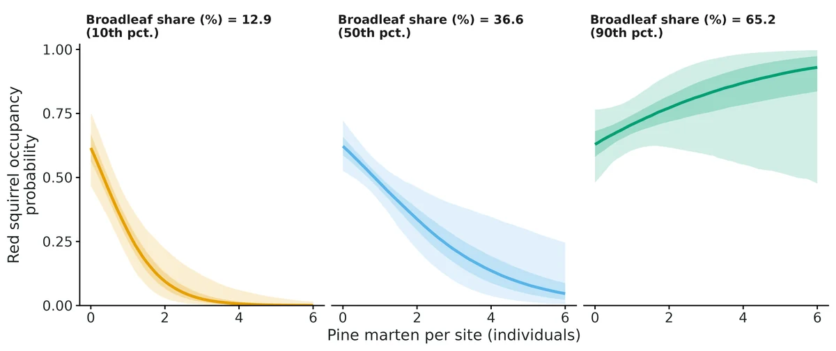
What this means
- Each 1-SD increase in woodland_pct (1 SD = 17.4 units) is associated with 1.70 (95% CI 1.47 to 1.96) times the expected Pine marten abundance (a +70% change) (per 10 units: rate ratio 1.36 (95% CI 1.25 to 1.47)).
- Interaction at average habitat: each additional Pine marten individual at a site is associated with 0.59 (95% CI 0.39 to 0.85) times the odds that Red squirrel occupies the site (odds ratio per individual); on the logit scale the coefficient is -0.53 (95% CI -0.93 to -0.17) per individual. The posterior probability that the association is negative is > 0.99.
- Predicted Red squirrel occupancy at average habitat: 0.62 (0.52-0.72) at a site with no Pine marten, 0.50 (0.42-0.57) with 1, 0.37 (0.25-0.49) with 2 and 0.26 (0.12-0.44) with 3 individuals (posterior medians, 95% CI).
- Habitat dependence: the interaction changes by 0.69 (95% CI 0.30 to 1.14) logit units per individual for each 1-SD (20.8 units) increase in broadleaf_pct; the 95% interval excludes zero, so the data support an interaction whose strength depends on habitat.
- Where broadleaf_pct = 12.9 (10th percentile): odds ratio per Pine marten individual 0.25 (95% CI 0.12 to 0.50) (negative).
- Where broadleaf_pct = 65.2 (90th percentile): odds ratio per Pine marten individual 1.42 (95% CI 0.84 to 2.53) (not clearly different from zero).
- Comparison with the common two-step shortcut (estimate Pine marten abundance first, then use it as a fixed covariate): the shortcut gives -0.48 (95% CI -0.81 to -0.15), with an interval 86% as wide as the joint model's. The joint model carries the uncertainty in each site's abundance into the interaction; the shortcut treats estimated abundance as if it were known, and in simulations it is biased towards zero with too-narrow intervals.
- Caution: this is an association between the dominant's estimated abundance and the subordinate's occupancy, not proof of predation or competition. Unmodelled habitat preferences shared (or opposed) by the two species produce the same signal, so include the main habitat drivers of both species. Royle-Nichols abundance assumes individuals are detected independently and abundance is Poisson among sites; absolute abundance is less reliable than relative differences. Simulation checks for this module (VALIDATION.md) recovered the interaction without bias at 600 sites (4 weekly occasions of daily records), including when the dominant's per-individual daily detection was as low as 0.03; in an independent check with 700 sites and a weaker interaction its size was overstated by about 12%, and with 150-300 sites by roughly 10-20% (credible intervals kept near-nominal coverage). With fewer than about 1000 sites, read the interval rather than the point estimate.
More figures
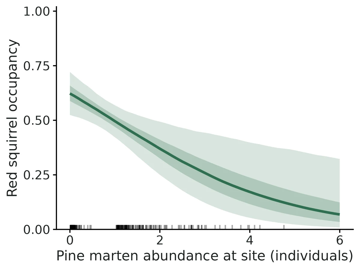
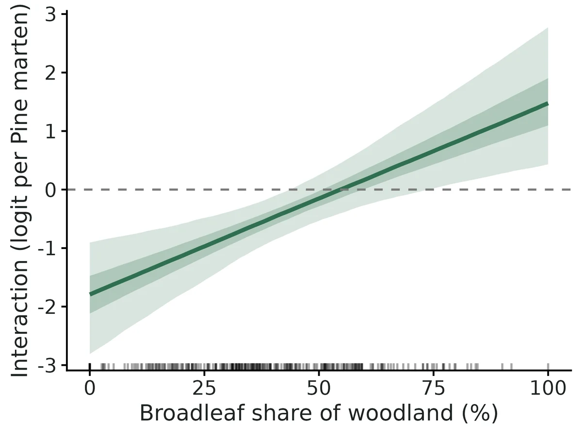
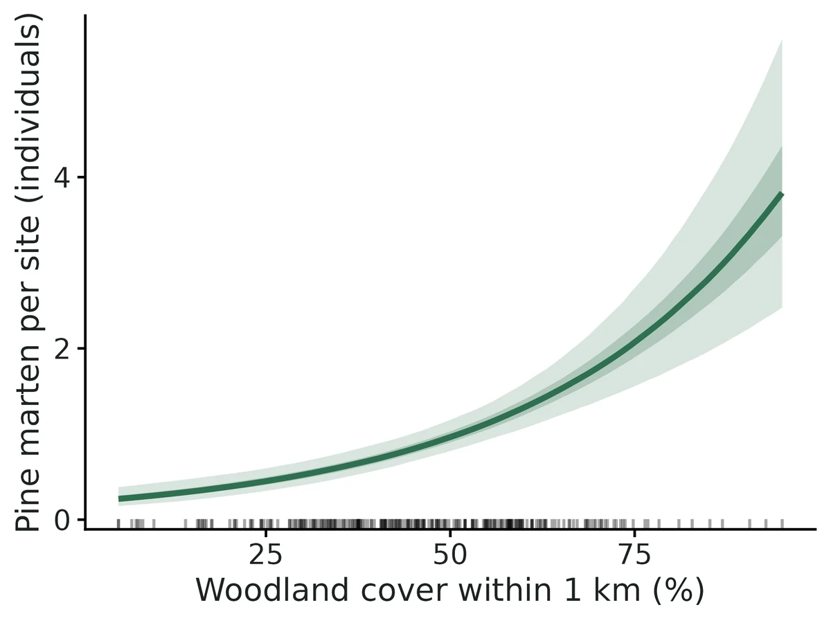
Figures are the module's default publication figures, reduced for the web. The report also saves them as PDF and full-resolution PNG.
Planted truth at the example's design
Before trusting the example's results, the module was run on many simulated data sets with the same design and known true values. Each row is one quantity: did the method get it back? (What the thresholds are.)
What OPEN means here. The module works (it passes at its default design), but at this example's design not every quantity passed the planted-truth check, so CascadiaTools does not certify those. 11 of the 12 quantities checked passed outright. For psi beta dominant abundance, the estimate was biased (by up to 11%); don't interpret those at this design. The quantities that passed can be used as reported. With your own data, the report would say the same and suggest what would help: more data, a simpler model or a different estimator. More on DONE and OPEN.
Why, for this example:
Planted truth at the example design (260 sites) fails for gamma0 (psi_beta_dominant_abundance): relative bias -11.0% (limit 10%; 3.2 MCSE) with coverage 0.95. Known limit 1 in VALIDATION.md. Convergence, GOF, cross-checks, negative control and reproducibility pass. Read the gamma0 interval, not its point estimate.
| This example | 260 camera sites, 4 weekly occasions, pine marten and red squirrel |
|---|---|
| Design the module was validated at | 600 camera sites, 4 weekly occasions |
The example has fewer than half the sites the module was validated at (260 vs 600). At 600 sites every occupancy coefficient was within 4% of the truth. At 300 sites the habitat-dependent interaction was overstated (+19.4% bias with Nimble, +11.3% with the independent maximum-likelihood engine on the same data), so this is finite-sample bias of the design, not a coding or MCMC problem. At the example's own 260 sites the occupancy coefficients carry roughly 10-20% bias: the marten-abundance effect -11.0% (fails), the broadleaf effect +21.8%, the woodland effect +10.2% and the habitat-by-interaction term +9.1% (all borderline passes). Coverage stays 0.92-0.96, so read these intervals rather than the point estimates, and use 600 or more sites for a new study.
These calls sit close to the pass/fail line. With another 100 simulated data sets they could come out the other way, so read them as “about at the limit” rather than as a clear pass or fail. Where the allowance is set by the noise floor, a quantity with a small true value can pass with a larger percentage bias than a quantity that fails. PASS there means the bias could not be told apart from simulation noise, not that the quantity is estimated better.
- psi_beta_broadleaf (✓ PASS): bias +21.8% against an allowance of ±23.2% (set by the simulation-noise floor (3 Monte Carlo SE)), so it used 94% of the allowance.
- psi_beta_dominant_abundance (✗ FAIL): bias -11.0% against an allowance of ±10.4% (set by the simulation-noise floor (3 Monte Carlo SE)), so it used 105% of the allowance.
- psi_beta_dominant_abundance_x_broadleaf (✓ PASS): bias +9.1% against an allowance of ±11.0% (set by the simulation-noise floor (3 Monte Carlo SE)), so it used 83% of the allowance.
- psi_beta_woodland (✓ PASS): bias +10.2% against an allowance of ±12.7% (set by the simulation-noise floor (3 Monte Carlo SE)), so it used 80% of the allowance.
11 of 12 rows pass; 4 are borderline.
| Quantity | True value | Average estimate | Bias | Allowed bias | Coverage (needed) | Result |
|---|---|---|---|---|---|---|
| dominant_detection_per_individual | 0.08 | 0.0814 | +1.7% | ±10.0% | 0.97 (0.885) | ✓ PASS |
| dominant_mean_abundance | 1 | 0.986 | -1.4% | ±10.0% | 0.96 (0.885) | ✓ PASS |
| dominant_prop_occupied | 0.63 | 0.629 | -0.2% | ±10.0% | 0.92 (0.885) | ✓ PASS |
| dominant_total_abundance | 293.6 | 292.8 | -0.3% | ±10.0% | 0.98 (0.885) | ✓ PASS |
| lambda_beta_woodland | 0.5 | 0.507 | +1.5% | ±10.0% | 0.94 (0.885) | ✓ PASS |
| psi_beta_broadleaf | 0.3 | 0.365 | +21.8% | ±23.2%† | 0.95 (0.885) | ✓ PASS ≈ borderline |
| psi_beta_dominant_abundance | -0.6 | -0.666 | -11.0% | ±10.4%† | 0.95 (0.885) | ✗ FAIL ≈ borderline |
| psi_beta_dominant_abundance_x_broadleaf | 0.6 | 0.655 | +9.1% | ±11.0%† | 0.96 (0.885) | ✓ PASS ≈ borderline |
| psi_beta_woodland | 0.5 | 0.551 | +10.2% | ±12.7%† | 0.92 (0.885) | ✓ PASS ≈ borderline |
| subordinate_detection | 0.15 | 0.15 | +0.2% | ±10.0% | 0.95 (0.885) | ✓ PASS |
| subordinate_occupancy_no_dominant | 0.6 | 0.61 | +1.6% | ±10.0% | 0.92 (0.885) | ✓ PASS |
| subordinate_prop_occupied | 0.464 | 0.465 | +0.2% | ±10.0% | 1 (0.885) | ✓ PASS |
Limits that matter
- 260 sites is below the ~600 sites validated for a habitat-dependent interaction; at this design gamma0 is overstated by ~11% (coverage stays 0.95). Read intervals, not point estimates.
- The broadleaf main effect on red squirrel occupancy is weakly identified at this design (planted-truth power 0.34).
- Association, not causation: unmodelled habitat shared by both species loads onto the interaction term.
- Royle-Nichols assumptions (Poisson abundance, independent detection of individuals, closure over 4 weeks) were not stress-tested; group-living or overdispersed martens would bias abundance and the interaction. The posterior predictive check is the only guard.
- Abundance is the number of martens using a camera site, not a density; one marten can use several sites.
- The two-step plug-in shortcut fails the gate (attenuated, overconfident) and is shown for comparison only.
All known limits from the module's validation record
- Fewer than ~600 sites with a habitat-varying interaction. At 300 sites gamma1 is biased +19% (Nimble) / +11% (ML on the same data), and the gate fails. At 150 sites the biases are -18% (gamma0) and +23% (gamma1). Interval coverage stays near nominal, so CrIs can still be read. The point estimate overstates the strength of the interaction. A constant interaction (no habitat term) is better determined, but it was not separately gate-tested below 600 sites.
- Dominant per-individual detection at the default (r = 0.10) at 300 sites: coverage of r was 0.86 (bound 0.885). At 600 sites it is 0.93.
- Low dominant detection (r = 0.03/day) passes at 600 sites. Lower values and fewer sites were not tested. Expect interactions to be weakly identified there, and look at the width of the CrI.
- Royle-Nichols assumptions (Poisson N, independent and identical detection of individuals, closure) were not stress-tested. Overdispersed or group-living dominants will bias N_i and so gamma. The posterior predictive check is the only guard, and its power was not measured.
- Direction and causality: the model assumes A affects S's occupancy and that S's detection does not depend on N_A. Shared unmodelled habitat drivers load onto gamma. Reports state "associated with", not "caused by".
- Two-step engine fails the gate (attenuated, overconfident). It is shown for comparison only.
- Run time: about 6 min per Nimble fit at 600 sites with fast settings (1 core per replicate); the full default settings took 7.7 min at 260 sites (4 cores, incl. GOF and two-step). Scale roughly linearly in sites.
- Not implemented: abundance (N-mixture) model for the subordinate; time-varying (dynamic) interactions; more than two species; spatially explicit N (SCR) for the dominant; covariates on the subordinate's detection that involve N_A.
How this module was validated
- 100 simulated data sets per design fitted with Nimble (3 chains x 5000 iterations, 1500 burn-in) and with an exact ML engine on the same data; all 12 quantities passed on both engines at 600 sites.
- A harder low-detection design (weekly detection about 0.19 for one marten) passed all 12; a smaller 300-site design failed on the habitat-by-interaction term (+19.4%).
- Negative controls: a presence-only interaction model fitted to abundance-driven data failed (interaction -49%, coverage 0.64); the common two-step shortcut was biased toward no interaction and overconfident. With no true interaction, false-positive rates were 0.08 and 0.03.
- Cross-checks: the dominant-species part matched unmarked::occuRN, and the reduced model matched the occu-single module within 0.015 on every parameter.
- Power for the habitat-dependent interaction: 0.70, 0.88 and 1.00 at 150, 300 and 600 sites, with magnitudes overstated by 13-23% below 600 sites.
- A separate verifier with its own simulator passed a 1400-site design, found a narrow failure (-11.6%) at 700 sites, confirmed the controls, and reproduced the builder's tables to every digit.
Every run uses the acceptance gate described on the validation page. The full record follows, section by section, exactly as kept in the module's VALIDATION.md.
Settings and pass/fail rule used for every run
All recovery runs: bin/Rscript core/run.R recover abund-interactions --config dev/abund-interactions/<cfg>.yaml --nsim 100 --cores 16 --out results/abund-interactions/recover_<cfg> (configs in dev/abund-interactions/; tables printed by dev/abund-interactions/val_tables.R straight from the saved *_recovery.rds, so no number below was typed by hand). Runs were made 2026-10-18/19 with R 4.5.3, nimble 1.4.3 and unmarked (ecotools Rlib/), on njobvu with 16 workers.
Recovery uses fast_settings: Nimble 3 chains x 5000 iterations, 1500 burn-in, thin 2 (5250 draws), no GOF and no two-step side fit. Replicate r uses seed 100000 + r. The Nimble, ML and two-step runs of a design therefore fit identical data sets (paired comparisons below).
Gate (core recovery_gate, unchanged): |bias| <= max(10% of |truth|, 3 MC SE), or <= max(0.1 x empirical SD, 3 MC SE) when truth = 0; coverage of the 95% interval >= 0.95 - 3 MC SE (0.885 at nsim 100); >= 90% of replicates converged. Nimble "converged" means max R-hat < 1.05 over all monitored quantities. The real-data standard printed in reports (R-hat < 1.01, bulk ESS >= 400) is checked separately on every fit.
Default design (module defaults): 600 camera sites; 4 occasions of 7 camera-days each, with 10% of occasions losing a random number of days. Dominant species: mean 1 individual per site at average woodland, log-slope on woodland 0.5, per-individual daily detection r = 0.10 (weekly ~0.52 for one individual). Subordinate: occupancy 0.6 where the dominant is absent, logit slopes woodland 0.5 and broadleaf 0.3, interaction gamma0 = -0.7 per dominant individual at average broadleaf share and gamma1 = +0.5 per SD of broadleaf share (the interaction weakens, then reverses, in broadleaf-rich woodland, as in Twining et al. 2022 Proc R Soc B), daily detection 0.15. Simulated with the model in README.md (Royle-Nichols with K camera-days per occasion), as in Twining et al. (2025) simulation I.
Verdict
| design / check | engine | result | |
|---|---|---|---|
| default (600 sites) | nimble (joint) | PASS all 12 estimands; 100/100 R-hat < 1.05 (max 1.012) | |
| default | ml (exact marginal likelihood, independent code) | PASS all 12 | |
| harder: low dominant detection (r = 0.03/day, ~0.19/week) | nimble | PASS all 12; 99/100 converged | |
| false-positive rate (gamma0 = gamma1 = 0) | nimble | PASS; P(95% CrI excludes 0) = 0.08 (gamma0), 0.03 (gamma1) | |
| negative control: occupancy-mediated model (psi depends on 1[N_A > 0]) fitted to abundance-mediated data | ml | FAIL (as required): gamma0 -49%, gamma1 +52%, psi_beta_woodland -27%; coverage 0.64 / 0.82 / 0.70 | |
| comparison: two-step plug-in (occuRN -> E[N\ | y] -> occu) | twostep | FAIL: gamma0 attenuated +11.6% (coverage 0.84), gamma1 -16.9% (0.87); intervals 13-14% too narrow |
| smaller: 300 sites | nimble | FAIL gamma1 (+19.4% bias) and r coverage 0.86 (others pass) | |
| smaller: 300 sites | ml | FAIL gamma1 (+11.3% bias) | |
| cross-check vs unmarked occuRN + occu-single module (one data set) | nimble vs ml vs unmarked | agree within 0.05 SD-units on all shared parameters (section 5) | |
| power over n_sites (150 / 300 / 600; nsim 50) | nimble | power for gamma1 0.70 / 0.88 / 1.00 (section 6) |
The module is DONE at the default design (600 sites, 4 weekly occasions, daily records). Smaller designs fail the bias rule for the habitat-by-interaction term. That is reported as a limit, and no threshold was changed.
Honesty note on the default design: the first full runs used 300 sites as the default (folders results/abund-interactions/n300_recover_*). There gamma1 was biased +19% (Nimble) and +11% (ML on the same data), so the joint model failed the gate. The ML engine shows the same direction of bias, so it is finite-sample bias of the estimator at that design, not an MCMC problem. The default was raised to 600 sites, the smallest design in the power run with |bias| < 10% for both interaction terms. Twining et al. (2025) also report that a habitat-varying interaction needs > 600 sites when occasions are single 0/1 records. The 300-site results stay in this file.
1. Recovery at the default design (600 sites)
nimble, joint model (nsim 100, 0 errors, 100/100 R-hat < 1.05, max R-hat 1.012, median 349 s per replicate on 1 core)
| param | truth | mean est | rel. bias | bias MCSE | coverage (bound) | CI width | mean post. SD | emp. SD | power | gate |
|---|---|---|---|---|---|---|---|---|---|---|
| dominant_detection_per_individual | 0.1 | 0.101 | +0.6% | 0.000496 | 0.93 (0.885) | 0.0188 | 0.0048 | 0.00496 | - | PASS |
| dominant_mean_abundance | 1 | 0.997 | -0.3% | 0.00561 | 0.97 (0.885) | 0.236 | 0.0603 | 0.0561 | - | PASS |
| dominant_prop_occupied | 0.632 | 0.632 | -0.0% | 0.000668 | 0.96 (0.885) | 0.0267 | 0.00688 | 0.0189 | - | PASS |
| dominant_total_abundance | 678 | 676 | -0.2% | 3.16 | 0.95 (0.885) | 117 | 30 | 35.7 | - | PASS |
| lambda_beta_woodland | 0.5 | 0.492 | -1.6% | 0.00435 | 0.98 (0.885) | 0.173 | 0.0442 | 0.0435 | 1 | PASS |
| psi_beta_broadleaf | 0.3 | 0.29 | -3.3% | 0.0126 | 0.98 (0.885) | 0.547 | 0.139 | 0.126 | 0.61 | PASS |
| psi_beta_dominant_abundance | -0.7 | -0.709 | -1.3% | 0.0134 | 0.96 (0.885) | 0.51 | 0.13 | 0.134 | 1 | PASS |
| psi_beta_dominant_abundance_x_broadleaf | 0.5 | 0.519 | +3.8% | 0.0134 | 0.95 (0.885) | 0.511 | 0.131 | 0.134 | 1 | PASS |
| psi_beta_woodland | 0.5 | 0.514 | +2.9% | 0.0132 | 0.92 (0.885) | 0.452 | 0.115 | 0.132 | 0.98 | PASS |
| subordinate_detection | 0.15 | 0.15 | -0.2% | 0.000435 | 0.94 (0.885) | 0.0173 | 0.00442 | 0.00435 | - | PASS |
| subordinate_occupancy_no_dominant | 0.6 | 0.601 | +0.2% | 0.00379 | 0.94 (0.885) | 0.137 | 0.0349 | 0.0379 | - | PASS |
| subordinate_prop_occupied | 0.443 | 0.443 | +0.0% | 0.000358 | 0.96 (0.885) | 0.0137 | 0.0036 | 0.0215 | - | PASS |
Finite-sample quantities (dominant_total_abundance, *_prop_occupied) are compared with the realised latent states of each data set. Their posterior SD is (correctly) smaller than the between-data-set SD.
ml engine, same 100 data sets (exact marginal likelihood: N_i in 0..60 and z_i summed out; Wald intervals; median 62 s/rep)
| param | truth | mean est | rel. bias | bias MCSE | coverage (bound) | CI width | mean SE | emp. SD | power | gate |
|---|---|---|---|---|---|---|---|---|---|---|
| dominant_detection_per_individual | 0.1 | 0.0993 | -0.7% | 0.000502 | 0.93 (0.885) | 0.0189 | 0.00497 | 0.00502 | - | PASS |
| dominant_mean_abundance | 1 | 1.01 | +0.8% | 0.00576 | 0.97 (0.885) | 0.241 | 0.0634 | 0.0576 | - | PASS |
| dominant_prop_occupied | 0.632 | 0.633 | +0.1% | 0.000681 | 0.96 (0.885) | 0.0276 | 0.00718 | 0.019 | - | PASS |
| dominant_total_abundance | 678 | 684 | +1.0% | 3.26 | 0.94 (0.885) | 124 | 31.8 | 36.9 | - | PASS |
| lambda_beta_woodland | 0.5 | 0.494 | -1.2% | 0.00437 | 0.98 (0.885) | 0.173 | 0.0441 | 0.0437 | 1 | PASS |
| psi_beta_broadleaf | 0.3 | 0.29 | -3.2% | 0.0125 | 0.98 (0.885) | 0.542 | 0.138 | 0.125 | 0.6 | PASS |
| psi_beta_dominant_abundance | -0.7 | -0.691 | +1.2% | 0.0131 | 0.95 (0.885) | 0.503 | 0.128 | 0.131 | 1 | PASS |
| psi_beta_dominant_abundance_x_broadleaf | 0.5 | 0.498 | -0.4% | 0.0132 | 0.95 (0.885) | 0.501 | 0.128 | 0.132 | 1 | PASS |
| psi_beta_woodland | 0.5 | 0.511 | +2.2% | 0.0132 | 0.93 (0.885) | 0.451 | 0.115 | 0.132 | 0.98 | PASS |
| subordinate_detection | 0.15 | 0.15 | -0.2% | 0.000434 | 0.94 (0.885) | 0.0173 | 0.00456 | 0.00434 | - | PASS |
| subordinate_occupancy_no_dominant | 0.6 | 0.601 | +0.1% | 0.00381 | 0.94 (0.885) | 0.137 | 0.0345 | 0.0381 | - | PASS |
| subordinate_prop_occupied | 0.443 | 0.443 | +0.0% | 0.000362 | 0.94 (0.885) | 0.0137 | 0.00362 | 0.0215 | - | PASS |
2. Harder design: low detection of the dominant (r = 0.03 per individual per day)
Config dev/abund-interactions/hard_lowdet.yaml; everything else at the default. One marten is then detected in a given week with probability ~0.19 instead of ~0.52, so N_i is much less certain.
nimble (nsim 100, 0 errors, 99/100 R-hat < 1.05; the exception had max R-hat 1.058; median R-hat_max 1.011; median 325 s/rep)
| param | truth | mean est | rel. bias | bias MCSE | coverage (bound) | CI width | mean post. SD | emp. SD | power | gate |
|---|---|---|---|---|---|---|---|---|---|---|
| dominant_detection_per_individual | 0.03 | 0.0313 | +4.3% | 0.000348 | 0.939 (0.884) | 0.0136 | 0.00347 | 0.00346 | - | PASS |
| dominant_mean_abundance | 1 | 0.982 | -1.8% | 0.0122 | 0.919 (0.884) | 0.446 | 0.114 | 0.121 | - | PASS |
| dominant_prop_occupied | 0.632 | 0.623 | -1.4% | 0.00327 | 0.929 (0.884) | 0.122 | 0.0312 | 0.0393 | - | PASS |
| dominant_total_abundance | 678 | 666 | -1.7% | 7.99 | 0.919 (0.884) | 282 | 71.9 | 82 | - | PASS |
| lambda_beta_woodland | 0.5 | 0.491 | -1.8% | 0.00569 | 0.97 (0.884) | 0.217 | 0.0555 | 0.0566 | 1 | PASS |
| psi_beta_broadleaf | 0.3 | 0.294 | -1.9% | 0.0148 | 0.97 (0.884) | 0.614 | 0.157 | 0.147 | 0.556 | PASS |
| psi_beta_dominant_abundance | -0.7 | -0.714 | -2.0% | 0.0159 | 1 (0.884) | 0.663 | 0.169 | 0.158 | 1 | PASS |
| psi_beta_dominant_abundance_x_broadleaf | 0.5 | 0.527 | +5.3% | 0.0153 | 0.96 (0.884) | 0.632 | 0.161 | 0.152 | 0.96 | PASS |
| psi_beta_woodland | 0.5 | 0.511 | +2.2% | 0.0159 | 0.889 (0.884) | 0.512 | 0.131 | 0.158 | 0.98 | PASS |
| subordinate_detection | 0.15 | 0.15 | -0.2% | 0.000431 | 0.929 (0.884) | 0.0173 | 0.00442 | 0.00428 | - | PASS |
| subordinate_occupancy_no_dominant | 0.6 | 0.599 | -0.2% | 0.00438 | 0.96 (0.884) | 0.17 | 0.0434 | 0.0436 | - | PASS |
| subordinate_prop_occupied | 0.443 | 0.443 | +0.0% | 0.000359 | 0.96 (0.884) | 0.0137 | 0.00359 | 0.0216 | - | PASS |
What low detection costs: the CrI for the dominant's total abundance is 2.4x wider (282 vs 117). The interaction intervals are 24-30% wider (gamma0 0.663 vs 0.51; gamma1 0.632 vs 0.511). Power for gamma1 falls from 1.00 to 0.96. The joint model widens its intervals (gamma0 coverage 1.00) instead of becoming biased. psi_beta_woodland coverage, 0.889, sits just above its bound of 0.884.
3. False-positive rate: no interaction (gamma0 = gamma1 = 0)
Config dev/abund-interactions/null_effect.yaml. nimble (nsim 100, 0 errors, 100/100 converged, median 350 s/rep)
| param | truth | mean est | bias | bias MCSE | coverage (bound) | CI width | power (= FPR) | gate |
|---|---|---|---|---|---|---|---|---|
| psi_beta_dominant_abundance | 0 | 0.011 | +0.011 | 0.0102 | 0.92 (0.885) | 0.394 | 0.08 | PASS |
| psi_beta_dominant_abundance_x_broadleaf | 0 | 0.0137 | +0.014 | 0.00895 | 0.97 (0.885) | 0.36 | 0.03 | PASS |
All other estimands pass as well (full table in results/abund-interactions/recover_null_effect/). The FPR of 0.08 for gamma0 lies within Monte Carlo error of 0.05: the binomial SE at nsim 100 is 0.022, so the 95% range is 0.01-0.09. Pooled over both terms, 11 of 200 tests rejected (0.055).
4. Negative control and the two-step shortcut (the gate CAN fail)
4a. Occupancy-mediated model fitted to abundance-mediated data (Twining et al. 2025, their central result)
Config occmediated.yaml: engine: ml, mediator: occupancy. The subordinate's occupancy then depends only on whether the dominant is present (1[N_i > 0]), which is the assumption behind Waddle et al. (2010) and Rota et al. (2016) style interaction models. The data are the same 100 default data sets.
| param | truth | mean est | rel. bias | coverage (bound) | gate |
|---|---|---|---|---|---|
| psi_beta_dominant_abundance | -0.7 | -1.05 | -49.4% | 0.64 (0.885) | FAIL (bias, coverage) |
| psi_beta_dominant_abundance_x_broadleaf | 0.5 | 0.761 | +52.2% | 0.82 (0.885) | FAIL (bias, coverage) |
| psi_beta_woodland | 0.5 | 0.364 | -27.2% | 0.70 (0.885) | FAIL (bias, coverage) |
| psi_beta_broadleaf | 0.3 | 0.277 | -7.7% | 0.96 | PASS |
| dominant / detection parameters | <= 2.2% | >= 0.93 | PASS |
The gate fails, as required. A presence-only interaction misstates the per-individual effect: the presence effect, -1.05, absorbs the effect of 1.6 individuals on average where martens are present. It also pulls the subordinate's woodland response towards zero, because woodland drives marten abundance. The same control at 300 sites fails in the same way (gamma0 -48.9%, gamma1 +67.1%, woodland -30.5%).
4b. Joint model vs two-step plug-in: does the joint model propagate the uncertainty in N_A?
The twostep engine fits unmarked::occuRN to the dominant and takes the empirical-Bayes posterior mean E[N_i | y]. It then fits unmarked::occu to the subordinate with that as a fixed covariate. This is the common shortcut. It runs on the same 100 default data sets as section 1 (median 4 s/rep):
| param | joint nimble: mean est / coverage / CI width | two-step: mean est / coverage / CI width | two-step gate |
|---|---|---|---|
| psi_beta_dominant_abundance (truth -0.7) | -0.709 / 0.96 / 0.510 | -0.619 / 0.84 / 0.443 | FAIL (bias +11.6%, coverage) |
| psi_beta_dominant_abundance_x_broadleaf (truth 0.5) | 0.519 / 0.95 / 0.511 | 0.416 / 0.87 / 0.437 | FAIL (bias -16.9%, coverage) |
| psi_beta_woodland (0.5) | 0.514 / 0.92 / 0.452 | 0.506 / 0.93 / 0.446 | PASS |
Paired on identical data (n = 100): the two-step interval is narrower in the median data set, by 0.869x the joint width for gamma0 and 0.858x for gamma1. The two-step point estimates correlate 0.92-0.94 with the joint ones but are shrunk towards zero. This is classical errors-in-variables attenuation: E[N|y] is a noisy, shrunk proxy for N. Ignoring that noise makes the shortcut both biased towards "no interaction" and overconfident. The joint model gets both right. At 300 sites the two-step gamma0 is again attenuated (+10.6%, coverage 0.87). Every report shows the two-step fit beside the joint fit (compare_twostep: TRUE, figure joint_vs_twostep) but never uses it for inference.
5. Cross-checks against independent implementations (single data sets)
Script dev/abund-interactions/crosscheck.R, log logs/abund-interactions_crosscheck.log, tables in results/abund-interactions/crosscheck/. It uses K = 1 (6 plain 0/1 occasions, 300 sites), so unmarked's occuRN and occu fit exactly the same observation model.
A. Interaction present (seed 7; r = 0.3, p = 0.4). Columns give the estimate (95% interval). Nimble: R-hat max 1.001, min ESS 2602; posterior predictive Bayesian p = 0.53 for the dominant and 0.39 for the subordinate.
| param | truth | nimble joint | ml (own code) | two-step | unmarked occuRN |
|---|---|---|---|---|---|
| dominant_mean_abundance | 1 | 1.10 (0.91, 1.32) | 1.12 (0.92, 1.35) | 1.12 | 1.12 (0.92, 1.35) |
| lambda_beta_woodland | 0.5 | 0.469 (0.339, 0.597) | 0.473 (0.344, 0.601) | 0.465 | 0.465 (0.336, 0.594) |
| dominant_detection_per_individual | 0.3 | 0.282 (0.239, 0.326) | 0.277 (0.235, 0.323) | 0.278 | 0.278 (0.235, 0.325) |
| psi_beta_dominant_abundance | -0.7 | -0.662 (-1.08, -0.30) | -0.622 (-1.00, -0.25) | -0.613 (-0.95, -0.28) | - |
| psi_beta_dominant_abundance_x_broadleaf | 0.5 | 0.604 (0.196, 1.09) | 0.542 (0.112, 0.972) | 0.502 (0.132, 0.871) | - |
| interaction_at_low_broadleaf | -1.39 (-2.21, -0.70) | -1.28 (-2.01, -0.55) | -1.22 (-1.84, -0.60) | - | |
| interaction_at_high_broadleaf | 0.104 (-0.48, 0.70) | 0.066 (-0.49, 0.62) | 0.023 (-0.48, 0.53) | - | |
| psi_beta_woodland | 0.5 | 0.694 | 0.672 | 0.673 | - |
| subordinate_detection | 0.4 | 0.400 | 0.401 | 0.401 | - |
| subordinate_occupancy_no_dominant | 0.6 | 0.580 | 0.576 | 0.583 | - |
The dominant-species part of the ML engine reproduces unmarked::occuRN to 2-3 significant figures. Nimble posterior means differ from the MLEs by at most 0.06 on the logit scale (< 0.3 posterior SD), as expected for skewed posteriors under weak priors. On this one data set the two-step interval for gamma1 is 0.74 wide, against 0.89 for the joint model.
B. Interaction = 0: the reduced model equals single-species occupancy (seed 8; data simulated with gamma = 0). Nimble with interaction: false (gamma fixed at 0) vs the occu-single module (unmarked engine) on the subordinate's detection histories, and vs unmarked::occuRN on the dominant's:
| param | truth | reduced nimble (95% CrI) | occu-single / occuRN (95% CI) | full joint (gamma free) |
|---|---|---|---|---|
| subordinate_occupancy_no_dominant | 0.6 | 0.586 (0.520, 0.651) | 0.584 (0.518, 0.648) | 0.556 |
| psi_beta_woodland | 0.5 | 0.894 (0.595, 1.23) | 0.880 (0.573, 1.19) | 0.849 |
| psi_beta_broadleaf | 0.3 | 0.315 (0.046, 0.601) | 0.309 (0.036, 0.581) | 0.308 |
| subordinate_detection | 0.4 | 0.423 (0.391, 0.456) | 0.424 (0.391, 0.458) | 0.423 |
| dominant_mean_abundance | 1 | 1.05 | 1.06 | 1.04 |
| lambda_beta_woodland | 0.5 | 0.425 | 0.427 | 0.426 |
| dominant_detection_per_individual | 0.3 | 0.296 | 0.293 | 0.298 |
The reduced model matches occu-single and occuRN to within 0.015 on every parameter. The full joint model fitted to the same null data estimates gamma0 = 0.116 (95% CrI -0.197, 0.440), which correctly includes 0.
6. Power over number of sites
Output: results/abund-interactions/power_sites/ (Nimble, fast settings, all other values at the default).
| n_sites | param | rel. bias | coverage | CI width | power | converged |
|---|---|---|---|---|---|---|
| 150 | psi_beta_dominant_abundance | -18.2% | 0.94 | 1.10 | 0.92 | 50/50 |
| 150 | psi_beta_dominant_abundance_x_broadleaf | +23.1% | 0.98 | 1.13 | 0.70 | 50/50 |
| 150 | dominant_mean_abundance | +0.6% | 0.96 | 0.477 | - | 50/50 |
| 150 | psi_beta_broadleaf | +2.7% | 1.00 | 1.16 | 0.18 | 50/50 |
| 300 | psi_beta_dominant_abundance | -13.4% | 0.94 | 0.762 | 1.00 | 50/50 |
| 300 | psi_beta_dominant_abundance_x_broadleaf | +15.9% | 0.94 | 0.773 | 0.88 | 50/50 |
| 300 | dominant_mean_abundance | -2.0% | 0.96 | 0.327 | - | 50/50 |
| 300 | psi_beta_broadleaf | +5.0% | 0.92 | 0.796 | 0.36 | 50/50 |
| 600 | psi_beta_dominant_abundance | -4.0% | 0.98 | 0.513 | 1.00 | 50/50 |
| 600 | psi_beta_dominant_abundance_x_broadleaf | +9.5% | 0.96 | 0.523 | 1.00 | 50/50 |
| 600 | dominant_mean_abundance | -1.9% | 0.92 | 0.232 | - | 50/50 |
| 600 | psi_beta_broadleaf | -7.4% | 0.96 | 0.545 | 0.56 | 50/50 |
Reading: with gamma0 = -0.7 per individual, the constant part of the interaction is detected (power >= 0.92) even at 150 sites. The habitat-dependence (gamma1 = 0.5 per SD) needs about 300 sites for 80% power and 600 for 100%. Below 600 sites both interaction terms are biased away from zero, by 13-23%: magnitudes are overstated, an effect that falls as n grows (the usual small-sample inflation of logistic coefficients, amplified by the latent covariate). Coverage stays >= 0.94 throughout, so intervals remain honest even where the point estimate is biased. With nsim 50, power and coverage have MC SE of about 0.03-0.07 and bias about 3-5%.
7. Example data set
example/ is a simulated pine marten - red squirrel camera survey in the formats camera-trap software exports: deployments.csv (with gaps and re-deployments), records.csv (timestamped detections of several species, including non-target ones) and sites.csv. It has 260 sites, up to 28 camera-days each, and truth in example/TRUTH.md. core/run.R fit on example/config.yaml (default settings: 3 x 20 000 iterations, GOF, two-step comparison) took 7 min 41 s on 4 cores. It gives results/abund-interactions/example/abund-interactions_report.html: max R-hat 1.001, min bulk ESS 3279, posterior predictive p 0.51 (marten) and 0.32 (squirrel). Estimates against the simulation truth:
| quantity | truth | estimate (95% CrI) |
|---|---|---|
| gamma0, logit per marten at mean broadleaf | -0.6 | -0.53 (-0.93, -0.17) |
| gamma1, per SD broadleaf share | 0.6 | 0.69 (0.31, 1.14) |
| marten daily detection per individual | 0.08 | 0.084 (0.071, 0.098) |
| marten log-slope on woodland | 0.5 | 0.53 (0.39, 0.67) |
| squirrel occupancy with no marten | 0.6 | 0.62 (0.53, 0.72) |
| total marten-site abundance | 274 | 256 (224, 298) |
| proportion of sites with squirrel | 0.504 | 0.513 (0.500, 0.527) |
I read the report and every interpretation sentence matches the table. For example, odds ratio per marten exp(-0.53) = 0.59. At the 10th / 90th percentile of broadleaf share the odds ratio is 0.25 / 1.42, the second with a CrI overlapping 1, worded "not clearly different from zero". The two-step interval is 86% as wide as the joint one. The figures render on the response scale with 50% and 95% posterior bands: squirrel occupancy vs marten abundance, interaction curves at the 10th/50th/90th percentile of broadleaf, interaction strength across broadleaf, abundance and occupancy vs woodland, abundance map, coefficients, joint vs two-step, GOF and trace. The example has 260 sites, below the validated 600, so the report carries the SMALL DESIGN note.
Independent verification (2026-10-19, separate verifier agent)
Done by an agent that did not build the module. Scripts are in dev/abund-interactions/verify/, saved results in results/abund-interactions/verify/, and logs in logs/abund-interactions_verify*.log. The gate is core recovery_gate with no threshold changes.
Literature. The model was checked line by line against Twining, Augustine, Royle & Fuller (2025, Ecology 106:e4468; PMC11725697):
- N_i^D ~ Poisson(lambda_i), with log(lambda_i) linear.
- y^D_ij ~ Binomial(K, 1 - (1 - r_ij)^N_i).
- z^S_i ~ Bernoulli(psi_i), with logit(psi_i) = beta X + gamma0 N_i + gamma1 N_i x cov_i.
- y^S_ij ~ Bernoulli(p z_i). The module generalises this to Binomial(K_ij, z_i p_ij) over camera-days.
The Nimble code (abi_nimble_code), the exact-likelihood engine (abi_site_loglik) and the simulator all implement this model.
- gamma0 is the slope at the standardised modifier = 0, which is average habitat.
- The paper's sample-size findings match the README. A constant interaction was unbiased at 300 sites x 4 occasions. A covariate-varying interaction was biased below 600 sites x 10 single 0/1 occasions and unbiased at 1000 sites.
- The paper's priors are "vague" and given only in its Appendix S1. The module's Logistic(0,1) and N(0, SD 2) priors are a reasonable weakly informative choice.
The simulator and fit share only the formula and standardisation conventions. The planted-truth check below uses a separately written simulator, so a shared bug would have shown up there.
Independent planted truth (verify_sim.R, written without module code; nsim 100 per run).
Design:
- 700 sites, 5 occasions x 5 camera-days.
- 8% of occasions entirely missing (NA) and 12% with partial effort.
- Raw covariates in percent, and the two covariates are correlated.
- The modifier (
conifer) is not in the psi formula, so the module has to add its main effect. - An occasion covariate (rain) on subordinate detection.
Parameters:
- Dominant abundance: lambda = 1.5 at the mean.
- Dominant detection r = 0.12 per day.
- Subordinate: psi0 = 0.5, p = 0.2.
- A weaker interaction with the opposite sign of habitat dependence: gamma0 = -0.4, gamma1 = -0.35.
| run | engine | result | gamma0 rel. bias (cov.) | gamma1 rel. bias (cov.) |
|---|---|---|---|---|
| 700 sites | nimble | FAIL 1 of 13: gamma0 bias -11.6% (limit 10%, MCSE 0.009); all else passes, 100/100 R-hat < 1.05 (max 1.014) | -11.6% (0.94) | -3.8% (0.92) |
| 700 sites, same data | ml | PASS all 13 | -7.0% (0.95) | +0.3% (0.95) |
| 1400 sites | nimble | PASS all 13 (max R-hat 1.015) | -3.2% (0.94) | -5.4% (0.98) |
| 1400 sites, same data | ml | PASS all 13 | -0.4% (0.94) | -2.7% (0.98) |
| null (gamma0 = gamma1 = 0), 700 sites | nimble | PASS all 13; FPR 0.01 (gamma0), 0.05 (gamma1) | bias -0.0002 | bias -0.009 |
All other estimands passed at 700 sites, with |bias| <= 3.6% and coverage 0.92-0.98. They include dominant abundance, total abundance, r, p, the rain effect on p, woodland and conifer slopes, and the proportions occupied.
The 700-site failure is the same finite-sample inflation of the interaction's magnitude that the builder found at 300 sites. It is not a coding error:
- The exact ML fit on the same data sets also overstates gamma0 (-7%).
- The bias disappears at 1400 sites.
- Coverage stays nominal.
- The posterior median is no better than the mean (-10.6% vs -11.2% on the first 48 replicates;
median_diag.R).
The pooled false-positive rate over both null terms is 6/200 = 0.03.
Builder's numbers reproduced. These reruns used the builder's own command: core/run.R recover ... --nsim 100 with default.yaml and occmediated.yaml.
- Default design, nimble: all 12 estimands pass. The table matches section 1 to every printed digit (identical seeds).
- Negative control (occupancy-mediated): fails as reported. gamma0 coverage 0.64, gamma1 coverage 0.82, woodland coverage 0.70.
- The gate can therefore fail. The builder's own null run gave an FPR of 0.08 / 0.03, and this independent null gave 0.01 / 0.05. Both are consistent with 0.05.
Usability.
core/run.R fitonexample/config.yamlwas rerun with the final code. It took about 8 min on 4 cores, with max R-hat 1.001, min ESS 3279 and estimates identical to section 7.Every interpretation sentence was checked by hand against the estimate table. Examples:
- Odds ratio exp(-0.53) = 0.59 (0.39-0.85).
- Per-10-unit rate ratio exp(0.531 x 10/17.4) = 1.36.
- Low/high-broadleaf odds ratios 0.25 / 1.42.
- Two-step interval width 86% of the joint interval.
- Predicted occupancy 0.62/0.50/0.37/0.26 for 0-3 martens.
- The wording is associational throughout ("is associated with"). Detection is labelled as a detection process. Results are on the response scale: odds ratios, rate ratios and probabilities.
- Every figure required by docs/FIGURES.md is present: subordinate_vs_dominant, interaction_by_habitat, dominant_abundance_<cov>, dominant_abundance_map and coefficients. So are interaction_strength, subordinate_occupancy, joint_vs_twostep, gof and trace. The curves agree with
fit$estimates, for example psi(N=0) = 0.62 and psi(N=1) = 0.50 at average habitat. The axes use original units. Messy data (
messy_test.R) gives clear, actionable messages for each problem tested:- NA in a covariate.
- A misspelled site id: the run stops with "did you mean 'NI010'?".
- A wrong column name: the message lists the columns that are present.
- An empty date.
- A dd/mm/yyyy date format.
- Species-name case.
- Trailing spaces: these are trimmed, with a warning.
- End date before start date.
- A misspelled modifier.
- An empty site id.
Changes made by the verifier (only R/io.R and R/report.R were changed; none affect the likelihood or the samplers, so the recovery results above stand):
read_data:fm$ppartial-matchedfm$psi, so leaving outp:silently gave detection the occupancy covariates. Fixed by using[[ ]].- Unknown keys under
formulas:now stop with an error. - A missing
formulas:section now gives a warning. - Site/species whitespace is trimmed.
- Empty dates or site ids, duplicate covariate rows and site-id typos are caught.
- Factor habitat modifier: the report said gamma0 applied "at average habitat". It now says "where habitat = <reference level>", and each contrast is worded with its level and reference.
- The detection unit is now "camera-day" or "survey occasion" as appropriate. "Multiplies the odds" was reworded to "is associated with ... times the odds".
Figures:
- The coefficient forest-plot caption now says the slopes are per 1 SD (the axis labels carry raw units) and uses "credible" or "confidence" according to the engine.
- The x-axis labels of the abundance map overlapped at 6-digit eastings. Fixed with 3 breaks and
check.overlap.
- The SMALL DESIGN note and the report caution now cite the 700-site independent result. The README not_for and Simulation sections say the same.
Verdict: VERIFIED_WITH_LIMITS.
- The module passes the gate at its default design (600 sites, builder) and at an independent 1400-site design.
- The negative control fails, and the FPR is about 0.05.
- At an independent 700-site design with a weaker interaction, the Nimble posterior mean overstates the interaction at average habitat by 11.6%, which is just outside the 10% rule. Coverage stays nominal.
- For a habitat-varying interaction with fewer than about 1000 sites, read the credible interval rather than the point estimate, and run a planted-truth check at the user's own design.
Engine, references and full details
Engine: nimble (joint Bayesian, default); ml (exact marginal likelihood, cross-check); twostep (unmarked occuRN + occu plug-in, comparison only).
References
- Twining JP, Augustine BC, Royle JA, Fuller AK (2025) Abundance-mediated species interactions. Ecology 106(1):e4468. doi:10.1002/ecy.4468
- Twining JP, Sutherland C, Reid N, Tosh DG (2022) Habitat mediates coevolved but not novel species interactions. Proc R Soc B 289:20212338. doi:10.1098/rspb.2021.2338
- Twining JP, Lawton C, White A, Sheehy E, Hobson K, Montgomery WI, Lambin X (2022) Restoring vertebrate predator populations can provide landscape-scale biological control of established invasive vertebrates: insights from pine marten recovery in Europe. Global Change Biology 28:5368-5384. doi:10.1111/gcb.16236
- Royle JA, Nichols JD (2003) Estimating abundance from repeated presence-absence data or point counts. Ecology 84:777-790.
- Waddle JH et al. (2010) A new parameterization for estimating co-occurrence of interacting species. Ecological Applications 20:1467-1475.
- Rota CT et al. (2016) A multispecies occupancy model for two or more interacting species. Methods Ecol Evol 7:1164-1173.
- Fiske I, Chandler R (2011) unmarked. J Stat Softw 43(10). de Valpine P et al. (2017) NIMBLE. J Comput Graph Stat 26:403-413.
