Abundance

Distance sampling (conventional, multiple-covariate and hierarchical)

"How many deer (birds, primates, tortoises...) are there per square kilometre and in my study area, and is density higher in some habitats?" Observers miss more animals the farther away they are. Distance sampling models how detection falls with distance (the detection function), estimates the share of animals within the truncation distance that were seen, and corrects the counts for the ones that were missed.

module id: distance! Example verdict: OPENestimates accurate · intervals too narrow

Is this the right analysis?

Use it when

Observers walked line transects or stood at points and recorded the distance (perpendicular for lines, radial for points) to every animal or group they detected, with detection falling off with distance; the question is how many animals there are per km2 and in the study area, and (optionally) whether density is associated with habitat measured per transect. Exact or binned distances, single or repeated visits, groups (clusters), strata.

Not for

Counts without distances (use nmixture), detection/non-detection (occu-single), individually identified animals (scr or capture-recapture), camera-trap distance sampling with snapshot moments (not implemented), surveys where animals on the line are missed (g(0) < 1, e.g. diving whales or cryptic birds: needs double-observer mrds, not implemented), spatial density surface models over a full study area (DSM; only covariate-based prediction to a grid is offered).

The data you need

Observations CSV (transect id, distance, optional group size, optional visit, optional observer/weather), transects CSV (id, line length or number of visits, stratum, habitat covariates; every surveyed transect, including those with no detections), study-area size (km2, per stratum) for abundance, optional prediction grid.

What the example's main data file looks like:

First 5 of 146 rows of `deer_observations.csv`.
transect_id	date	observer	perp_distance_m	group_size
MD01	2025-01-19	JK	61	4
MD01	2025-01-19	JK	83	2
MD01	2025-01-19	JK	88	1
MD01	2025-01-19	JK	96	5
MD02	2025-01-16	AB	3	4

Not sure? Use the finder to compare modules.

Try it

The worked example

Mule deer density on a winter range from line-transect distance sampling, with shrub-cover and road-distance effects (simulated data)

The question: How many mule deer are on the 360 km2 winter range (per km2 and in total, overall and in the north and south units), and is deer density higher where shrub cover is higher and farther from the highway?

The data are simulated, so the true answer is known and the analysis can be checked against it.

What the researcher typed

I have a mule deer line-transect survey in this folder: a file of deer groups seen with the perpendicular distance from the line (m), group size, observer and date; a file of the 36 transects with their length, management unit (north or south, 180 km2 each), shrub cover and distance to the highway; and a 1 km2 grid of the whole 360 km2 winter range with the same two habitat values. Please estimate how many deer there are per km2 and in total, for each unit and overall, and tell me whether deer are more common where shrub cover is higher and farther from the road. Check that the method works for a survey like mine before you trust it, and give me a report and figures I can put in a paper.

Run it yourself

Download the example data below and unzip it.
Open the unzipped folder in Claude Code (see Install).
Paste the prompt above. The agent checks the files, writes a plan, runs planted truth, fits the model and writes the report. You can compare your results with the ones below.

Download the example data (zip, 14 KB)

Contains deer_observations.csv, deer_transects.csv, study_area_grid.csv, the settings file (config.yaml), a description of the data and a step-by-step walkthrough.

Study design details

model	conventional distance sampling (Distance::ds: half-normal / hazard-rate + cosine adjustments, AIC model-averaged, R2 variance) + hierarchical distance sampling (unmarked::distsamp) for habitat effects
survey	line transects, single visit, exact distances
transects	36
transects with zero detections	1
line length km	1.89-4.10 (mean 3.19)
total line km	114.9
study area km2	360
strata	north 180 km2, south 180 km2
truncation m	400
detections	146
detections within truncation	145
deer counted	486
mean group size observed	3.33
observers	2
density covariates	shrub_cover_pct, road_dist_km
prediction grid cells	360

What the report says

Results from the example data

Figure: Expected mule deer density versus shrub cover from the hierarchical distance-sampling model (road distance at its mean), with 95% and 50% bands; points are rough per-transect densities. — Expected mule deer density versus shrub cover from the hierarchical distance-sampling model (road distance at its mean), with 95% and 50% bands; points are rough per-transect densities.

What this means

A group within 400 m of the line had probability 0.44 (95% CI 0.38 to 0.50) of being detected. Equivalently, the effective strip half-width is 175 m.
Density: 12.0 (95% CI 9.24 to 15.5) individuals per km2, which over the 360 km2 study area is 4,314 (95% CI 3,328 to 5,593) individuals.
This is 3.59 (95% CI 2.82 to 4.58) groups per km2 times a mean group size of 3.34 (95% CI 3.12 to 3.56).
By stratum: north 7.97 (95% CI 5.68 to 11.2) per km2; south 16.0 (95% CI 11.6 to 22.0) per km2.
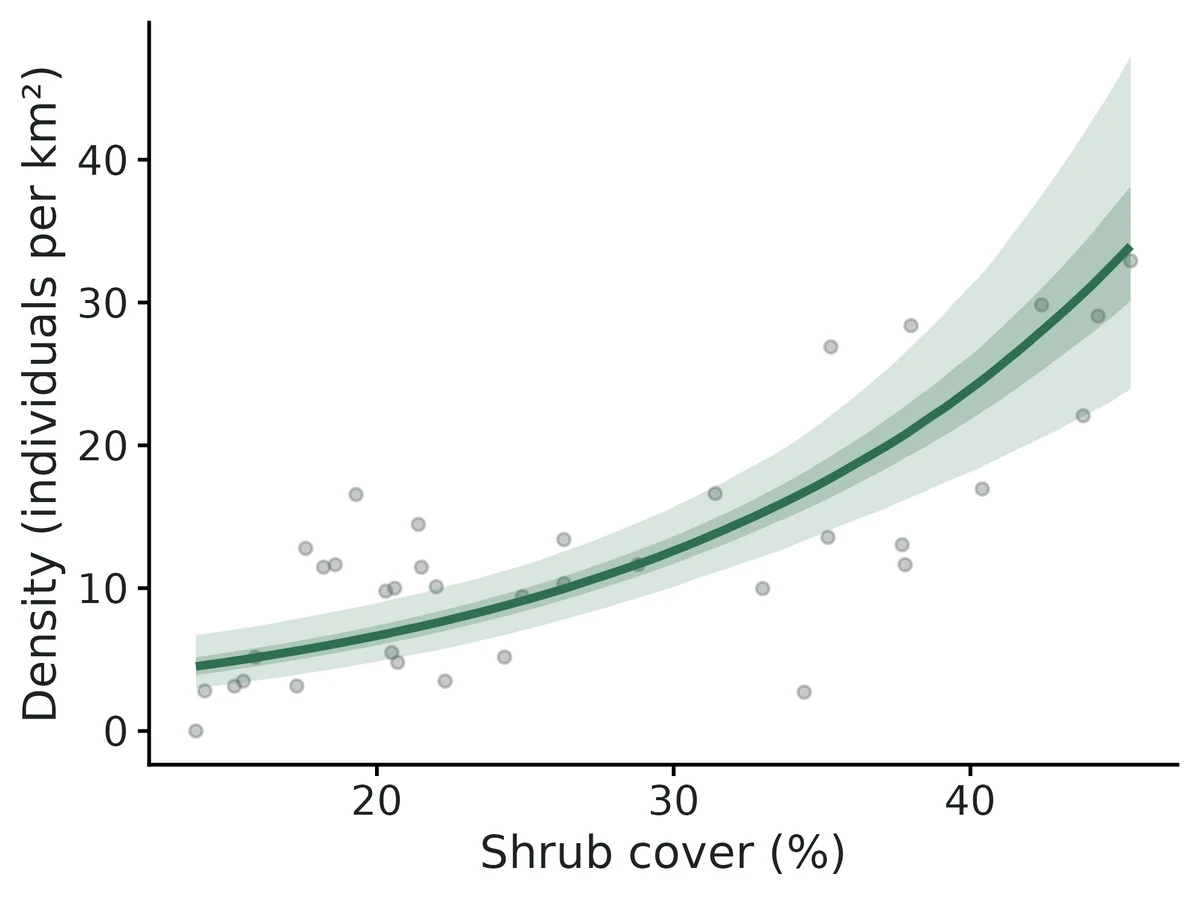
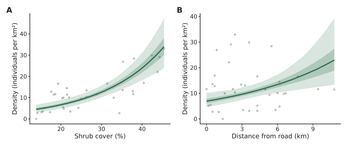
Each increase of 10 percentage points in shrub cover multiplies expected density by 1.89 (95% CI 1.56 to 2.30), i.e. +89%.
Each increase of 3 km in distance from road multiplies expected density by 1.40 (95% CI 1.12 to 1.74), i.e. +40%.
This is an association from an observational survey, not proof that shrub cover causes the difference.
The hierarchical model's density over the study area (12.2 (95% CI 9.70 to 15.3) per km2) agrees with the design-based estimate above.
Goodness of fit: Cramer-von Mises test of the distances, p = 0.72. No evidence of lack of fit.

More figures

Figure: Fitted half-normal detection function (model-averaged with hazard-rate) with 95% and 50% confidence bands over the histogram of the 145 perpendicular distances within 400 m, scaled to detection probability. — Fitted half-normal detection function (model-averaged with hazard-rate) with 95% and 50% confidence bands over the histogram of the 145 perpendicular distances within 400 m, scaled to detection probability.

Figure: Expected mule deer density versus distance from the highway (shrub cover at its mean), with 95% and 50% bands; points are rough per-transect densities. — Expected mule deer density versus distance from the highway (shrub cover at its mean), with 95% and 50% bands; points are rough per-transect densities.

Figure: Conditional effects of shrub cover (A) and road distance (B) on deer density. — Conditional effects of shrub cover (A) and road distance (B) on deer density.

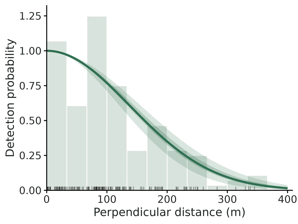
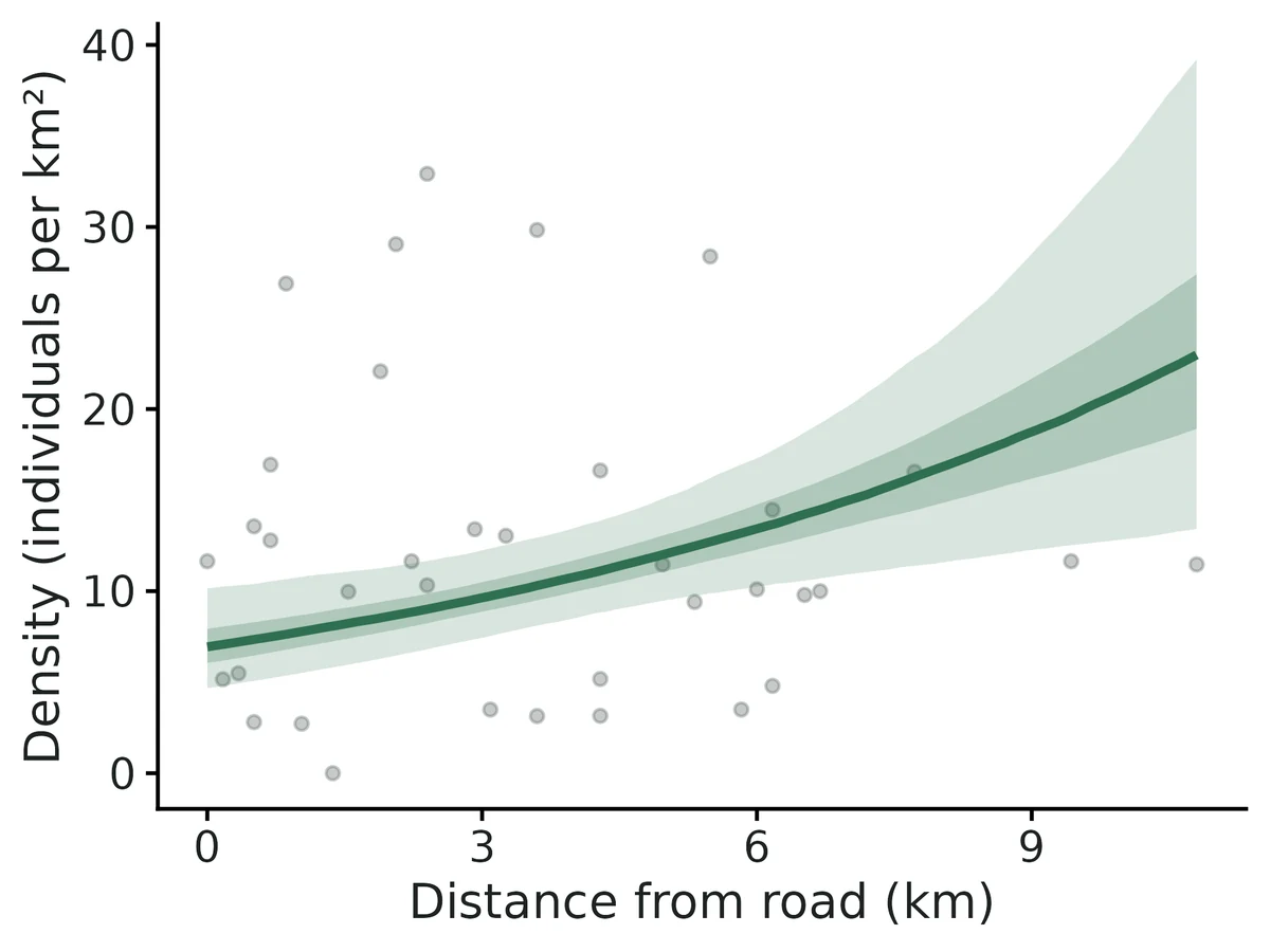
Figures are the module's default publication figures, reduced for the web. The report also saves them as PDF and full-resolution PNG.

How we know it works

Planted truth at the example's design

Before trusting the example's results, the module was run on many simulated data sets with the same design and known true values. Each row is one quantity: did the method get it back? (What the thresholds are.)

Verdict for this example: ! OPEN

What OPEN means here. The module works (it passes at its default design), but at this example's design not every quantity passed the planted-truth check, so CascadiaTools does not certify those. 11 of the 13 quantities checked passed outright. For density at average site, group density at average site, the estimate itself was accurate (within 10% of the truth on average), but the 95% interval was too narrow, containing the truth only 88% to 89% of the time. Use those estimates, but read their intervals as somewhat over-confident. The quantities that passed can be used as reported. With your own data, the report would say the same and suggest what would help: more data, a simpler model or a different estimator. More on DONE and OPEN.

Why, for this example:

All estimands that answer the question (density, abundance, per-unit density, detection, habitat rate ratio) pass planted truth at this design, the fit converged and both GOF checks pass; but the HDS density at an average transect (whose uncertainty also sets the bands on the conditional-effect curves and the map) under-covers (0.885 vs bound 0.904; VALIDATION.md Known limit 9, prepared fix not installed).

The example's design compared with the validated design: same as validated

This example	36 line transects (114.9 km), 145 detected mule-deer groups, 2 strata
Design the module was validated at	30 line transects of 3 km, median 145 detections

The example matches the validated default closely: a few more transects (36 vs 30) and the same median number of detections (145), with groups and two strata, which were validated separately. Density, abundance, detection and the habitat effect all passed at this design, but the density at an average transect from the habitat model under-covered (0.885 vs bound 0.904) because it ignores uncertainty in choosing the detection curve, a known limit with a prepared but uninstalled fix.

≈ Borderline results

These calls sit close to the pass/fail line. With another 200 simulated data sets they could come out the other way, so read them as “about at the limit” rather than as a clear pass or fail.

group_density_at_average_site (✗ FAIL): coverage 0.890 against a minimum of 0.904.

11 of 13 rows pass; 1 is borderline.

Bias: average estimate minus truth, as a percentage of the truth. Allowed bias: the largest bias that still passes, the bigger of 10% of the truth and 3 Monte Carlo standard errors († = set by that simulation-noise floor, so the allowance is wider than 10%). Coverage: share of 95% intervals that contained the true value, with the minimum needed in brackets. ≈ borderline: the bias used 80–125% of its allowance, or coverage was within 0.015 of the minimum; such a result could flip between PASS and FAIL with another set of simulations. Quantity names are as they appear in the report.
Quantity	True value	Average estimate	Bias	Allowed bias	Coverage (needed)	Result
abundance	4,193	4,149	-1.1%	±10.0%	0.97 (0.904)	✓ PASS
density_at_average_site	10.4	10.3	-0.5%	±10.0%	0.89 (0.904)	✗ FAIL
density_beta_habitat	0.49	0.488	-0.4%	±10.0%	0.95 (0.904)	✓ PASS
density_per_km2	11.7	11.5	-1.1%	±10.0%	0.97 (0.904)	✓ PASS
density_per_km2_S1	11.6	11.5	-1.3%	±10.0%	0.97 (0.904)	✓ PASS
density_per_km2_S2	11.7	11.6	-0.8%	±10.0%	0.98 (0.904)	✓ PASS
detection_prob	0.455	0.466	+2.4%	±10.0%	0.95 (0.904)	✓ PASS
esw_m	181.9	186.2	+2.4%	±10.0%	0.95 (0.904)	✓ PASS
group_density_at_average_site	3.05	3.04	-0.4%	±10.0%	0.89 (0.904)	✗ FAIL ≈ borderline
group_density_per_km2	3.43	3.4	-0.9%	±10.0%	0.99 (0.904)	✓ PASS
mean_group_size	3.4	3.39	-0.2%	±10.0%	0.93 (0.904)	✓ PASS
rate_ratio_habitat	1.63	1.64	+0.2%	±10.0%	0.95 (0.904)	✓ PASS
sigma_m	146	145.8	-0.1%	±10.0%	0.97 (0.895)	✓ PASS

Limits that matter

HDS intercept (density_at_average_site) ignores detection-key selection uncertainty: coverage 0.885 at this design (0.92 when half-normal chosen, as in this data set; 0.81 otherwise). Design-based density, abundance and slopes unaffected (Known limit 9).
Design-based density intervals are conservative when density follows habitat across transects (coverage 0.975 here; Known limit 3).
g(0) = 1, no evasive movement and accurate distances cannot be tested from these data; 75 m evasive movement biased density -27% in simulation, heaping at zero biased it upward (Known limit 4).
Recovery simulated one habitat covariate and a single detection scale; the second covariate (road) and the observer difference were checked only on the example fit.
The density map extrapolates to grid cells with shrub cover outside the surveyed 13.9-45.4 %.

All known limits from the module's validation record

Fewer than ~40 detections: the HDS intercept (density_at_average_site) under-covers (0.89 at 8 lines); with binned point data and a hazard-rate truth, density is biased +14% and the hazard-rate shape is not recoverable (section 2b, 2c). The report warns when < 60 detections.
gdistsamp (repeated visits) needs many transects and visits: +23% bias in density at 60 x 4, +5% at 120 x 6. Availability is weakly identified. If animals are sedentary between visits it fails badly (-29%); pool visits as effort with the single-visit engines instead.
Design-based intervals are conservative (coverage 0.98-0.99) when density follows a covariate trend across transects (R2/P2 behaviour), so they are wider than necessary.
g(0) = 1, no movement, accurate distances are untestable from the data alone: evasive movement gives -27% with coverage 0.45; heaping at 0 gives erratic upward bias (median +8%, 10% of datasets > 2x). How often the GOF test flags these violations was not measured.
The bootstrap variance option is slow (10-15 s per resample) and was validated only at the 12-line design (100 replicates).
MCDS detection-function figures show the curve averaged over covariates (no per-level curves).
Not implemented: double-observer (mrds, g(0) < 1), density surface models (DSM), camera-trap distance sampling, availability for diving or singing animals other than via repeated visits.
Observer-effect false-positive rate was 0.075 (15/200), borderline but within the binomial range.
HDS intercept ignores key-selection uncertainty (found in independent verification, below): density_at_average_site (and density_per_km2_hds) come from the AIC-best HDS key only. When the truth is half-normal the hazard-rate wins AIC in 20-30% of data sets, and the intercept interval then covers the truth in only 70-79% of them. At a 70-point design with 2 pooled visits overall coverage is 0.873 (FAIL, bound 0.897). Design-based density, abundance and the habitat slopes are unaffected. A fix is prepared but NOT installed or validated (see below).

How this module was validated

200 simulated data sets at the default design using Distance and unmarked; all 8 quantities passed, with design-based density intervals somewhat conservative (coverage 0.985).
Variants passed with 100 replicates each: groups with strata and observer effects, binned point transects, and repeated-visit surveys at 120 transects x 6 visits.
Harder designs: 12 lines passed; 8 lines (about 38 detections) failed one interval (coverage 0.890); sparse hazard-rate point data biased density +14.2%; 60 transects x 4 visits biased density +22.6%.
Negative controls: evasive movement (density -27.3%), heaping of distances at zero and sedentary animals across visits all failed; with no true effect, false-positive rates were 0.055 (habitat) and 0.075 (observer).
Cross-checks on 50 data sets per scenario: Distance and a hand-written likelihood agreed to better than 1e-6; unmarked's habitat model matched to 3.5e-5.
Power: about 50 lines (about 240 detections) give 80%+ power for a 28% density change per SD of habitat (0.77 at 30 lines).
A separate verifier with its own simulator passed independent line and point designs, found the key-selection coverage problem (0.873 in one point design), and fixed point-survey effort and data-entry checks.

Every run uses the acceptance gate described on the validation page. The full record follows, section by section, exactly as kept in the module's VALIDATION.md.

Settings and pass/fail rule used for every run

All runs: bin/Rscript core/run.R recover distance [--config dev/distance/rc_<label>.yaml] --nsim N --cores 16 (SLURM, 16 cores, njobvu or chinook) with the module fast_settings (keys hn + hr, cosine adjustments up to 2 by forward AIC, AIC model averaging, analytic variance; HDS derived quantities from 500 MVN draws; no GOF bootstrap). Raw results: results/distance/recover_<label>/ (summary CSV, per-replicate CSV, HTML report). Final runs: 2026-10-20 (code version with the HDS P_a-CV screen, see section 8). Gate (core/R/recovery.R::recovery_gate, thresholds unchanged):

bias	<= max(10% of truth, 3 MC SE); 95% interval coverage >= 0.95 - 3 MC SE (floor 0.80);

>= 90% of replicates converged (likelihood engines: optimiser converged, finite SEs, link-scale SE < 5).

Default design (module defaults): 30 line transects of 3 km, each in a 3 x 2 km cell (study area 180 km2); groups placed by an inhomogeneous Poisson process, density 4 / km2 at the average cell, log-density slope 0.4 per SD of a habitat covariate; half-normal detection, sigma = 150 m; exact distances simulated to 600 m and truncated at w = 400 m; single visit, no groups. This gives a median of 145 detections within w (IQR 137-155). Engine auto = Distance::ds (density, abundance, detection) + unmarked::distsamp (habitat effect, density at an average site).

Timing: selftest (4 reps) about 10-20 s per replicate; 100 replicates take 2-4 min on 16 cores.

sigma_m is reported only when the AIC-best model is a half-normal without adjustments, so its n is smaller than for the other estimands; hr_scale_m/hr_shape likewise only for a plain hazard-rate.

1. Recovery at the default design (nsim = 200) -- PASS

estimand	truth	mean est	rel. bias	coverage	power	gate
density_per_km2	4.32 (realised)	4.25	-1.6%	0.985		PASS
abundance	777.7	765.2	-1.6%	0.985		PASS
detection_prob (P_a)	0.466	0.480	+2.9%	0.935		PASS
esw_m	186.6	192.0	+2.9%	0.935		PASS
sigma_m (n = 144)	150	149.7	-0.2%	0.951		PASS
density_at_average_site (HDS)	4.00	3.96	-0.9%	0.930		PASS
density_beta_habitat (HDS)	0.40	0.395	-1.2%	0.920	0.995	PASS
rate_ratio_habitat (HDS)	1.492	1.491	-0.1%	0.920	0.995	PASS

200/200 converged, 0 failures, coverage bound 0.904. The design-based density interval is conservative (coverage 0.985): the R2 encounter-rate variance treats the covariate-driven trend in density between transects as random variation (Fewster et al. 2009 note the same for designs with trends).

Other variants at their own designs (nsim = 100)

MCDS + groups + strata (rc_mcds_clusters_strata: mean group size 3, observer B has log-sigma effect -0.3, 2 strata): all 14 estimands PASS. density -2.4% (cov 0.97), abundance -2.4% (0.97), density per stratum -0.3% / -4.3% (0.96 / 0.96), group density -2.1% (0.98), mean group size -0.2% (0.93), detection_beta_observerB -0.271 vs -0.300 (+9.6%, cov 0.94, power 0.48), P_a +3.6% (0.96), density_at_average_site -0.2% (0.89, bound 0.885), habitat slope 0.0% (0.93).

Point transects, binned (6 bins), half-normal (rc_point_binned_hn: 80 points, w = 150 m, sigma = 60 m, 20 groups / km2; median 38 detections): all 8 PASS, 100/100 converged. density +0.9% (cov 0.99), P_a +8.9% (0.97), edr_m +3.5% (0.97), density_at_average_site +5.7% (0.93), habitat slope +2.8% (0.96, power 0.72).

Point transects, binned, hazard-rate truth, 200 points (rc_point_binned_hr200, ~95 detections): all 9 PASS. density +8.9% (cov 0.96), P_a -4.8% (0.97), hr_shape +2.9% (n = 44, cov 1.00), habitat slope +3.9% (0.99, power 1.00).

Repeated visits, gdistsamp, 120 transects x 6 visits (rc_gds_big, availability 0.6): all 9 PASS. density +4.9% (cov 0.94), availability -2.6% (0.90), density_at_average_site +4.8% (0.95), habitat slope -0.4% (0.89), P_a +0.4% (0.96).

2. Harder designs (< 60 detections)

(a) 12 lines (rc_hard, median 58 detections; 57% of datasets have < 60) -- PASS, nsim = 200: density +1.7% (cov 0.99), P_a +2.4% (0.965), sigma +0.1% (0.97), density_at_average_site +2.8% (0.905, bound 0.904), habitat slope -3.2% (0.97, power 0.79).

Same design with variance: bootstrap (100 resamples of transects with full model selection in each; 4 x 25 replicates, seeds 11-14, pooled; 97/100 replicates converged): density -1.8% (cov 0.98), P_a +3.8% (0.91). Intervals are 21% wider than analytic ones at this design.

(b) 8 lines (rc_hard8, median 38 detections, all < 60) -- FAIL on one estimand, nsim = 200:

estimand	rel. bias	coverage	gate
density_per_km2 / abundance	+4.5%	0.965	PASS
detection_prob	+1.7%	0.935	PASS
density_at_average_site (HDS)	+1.6%	0.890 (bound 0.904)	FAIL
density_beta_habitat	+7.3%	0.925	PASS (power 0.60)

The HDS intercept interval (Wald, Poisson between-transect variation) is slightly too narrow with 8 transects. The design-based density remains valid.

(c) Binned points, hazard-rate truth, 80 points (rc_point_binned_hr, ~38 detections) -- FAIL: density +14.2% (cov 0.98), density_at_average_site +16.2% (0.94), hr_shape mean 9.9 vs 3 (n = 26, cov 0.73), hr_scale cov 0.77. P_a (-3.5%) and the habitat slope (+2.6%, cov 0.94) PASS. With 6 bins and ~38 detections the hazard-rate shoulder is not identified; AIC often picks the half-normal and density is biased upward. At 200 points (section 1) everything passes.

(d) gdistsamp, 60 transects x 4 visits (rc_gds) -- FAIL: density / abundance / density_at_average_site +22.6% (coverage 0.95-0.97, so the intervals are honest but very wide); availability -7.2% (0.98); habitat slope +0.1% (0.92), P_a +0.4% (0.93) PASS. Availability is weakly identified from visit-to-visit count variation; at 120 x 6 the bias drops to +4.9% (PASS).

3. Negative controls (the gate can fail)

scenario (nsim = 100)	density rel. bias	density coverage	P_a bias	gate
evasive movement 75 m before detection (`rc_nc_move`)	-27.3% (median -27%, 99% of reps < -10%)	0.45	+27.7% (cov 0.44)	FAIL density, abundance, P_a, ESW, density_at_average_site (cov 0.11)
heaping: distances < 60 m recorded as 0 (`rc_nc_heap`)	+336% mean (median +7.9%; 10% of reps > 2x truth)	0.90	-12.8% (cov 0.81)	FAIL density, abundance, P_a, ESW
gdistsamp with sedentary animals, same distance each visit (`rc_gds_fixed`, 93/100 converged)	-28.9%	0.31	+4.2% (cov 0.66)	FAIL density, abundance, availability (+32%), P_a

The habitat slope stays unbiased in all three (it is a ratio, and the violation affects all transects alike), which is the expected behaviour.

4. False-positive rate (effect = 0)

rc_null: density_beta_habitat = 0 and observer effect on sigma = 0 (MCDS fitted with ~ observer), nsim = 200. All estimands PASS. Rejection rate of the habitat effect = 0.055 (11/200; 95% CI on the rate 0.03-0.10), observer effect = 0.075 (15/200; 0.04-0.12). Both are consistent with the nominal 0.05 (the observer rate is borderline, Wald test with ~70 detections per observer).

5. Cross-checks against independent implementations

dev/distance/crosscheck.R (log logs/distance_crosscheck.log, CSV results/distance/crosscheck/): 50 datasets per scenario, half-normal key, no adjustments, fitted three ways: Distance::ds, unmarked::distsamp, and the module's hand-written likelihoods (R/engine_rlik.R: conditional distance likelihood for CDS, Poisson-multinomial likelihood for HDS, optim, no package code).

scenario	quantity	max abs. relative difference
lines, exact (60 lines)	sigma, P_a, density: Distance vs hand-coded	< 1e-6
	SE(density): Distance vs hand-coded (R2 + delta)	4.5%
	HDS beta: unmarked vs hand-coded	3.5e-5 (SE 4e-6)
	HDS density at average site: unmarked vs hand-coded	0.9% (draw-based)
	density: Distance vs unmarked HDS	mean +0.4%, SD 0.6%
points, binned (100 points)	sigma, P_a, density: Distance vs hand-coded	< 1e-6
	SE(density): Distance (P2) vs hand-coded	13%
	HDS beta: unmarked vs hand-coded	4e-4
	density: Distance vs unmarked HDS	mean +3.6%

The HDS likelihood was also checked term by term (dev/distance/hdscheck.R): my band probabilities and negative log-likelihood equal unmarked's to 7 digits for lines and points. The hand-coded engine also passes recovery on its own (rc_rlik, nsim = 100: density +1.3%, cov 1.00; P_a -0.2%, 0.97; sigma -0.1%, 0.97; habitat slope +0.1%, 0.91; all PASS).

6. Power

n_transects (3 km each)	10	20	30	50	80
power for density_beta_habitat	0.35	0.69	0.77	0.97	0.99
coverage of the slope	0.93	0.93	0.96	0.97	0.94
mean 95% CI width, density (/km2, truth ~4)	3.61	2.56	2.11	1.68	1.29

Report: results/distance/power/distance_power_report.html. About 50 lines (~240 detections) are needed for 80%+ power to detect a 28% change in density per SD of habitat.

7. Example fit

bin/Rscript core/run.R fit distance --config modules/distance/example/config.yaml --out results/distance/example (36 lines, 145 detected mule-deer groups): half-normal chosen (hazard-rate +1.9 AIC; model-averaged), P_a 0.44, ESW 175 m, density 12.0 / km2 (9.2-15.5), abundance 4,314 (3,328-5,593), CvM p = 0.72; HDS shrub-cover rate ratio 1.87 per SD (1.54-2.26), road-distance 1.36 (1.11-1.66); the HDS density over the prediction grid (12.2 / km2) agrees with the design-based estimate. I checked the interpretation sentences against the table (per-10-pp shrub effect exp(0.624 x 10/9.78) = 1.89) and looked at all 8 PNG figures. config_mcds.yaml (observer on sigma) gives density 11.9 / km2 and an observer-JK scale ratio of 0.85 (0.65-1.10).

8. Fix made during validation

The first round showed density_at_average_site in binned point transects (half-normal truth) with mean 107 vs truth 20: in 2 of 100 datasets the HDS chose a hazard-rate fitted as a near-spike to the 6 bands (P_a near 0, density 1,640 and 6,862 / km2) that passed the link-SE < 3 screen. The HDS engine now also drops a key whose average detection probability has CV > 50% when another key is stable (the rule Distance::ds candidates already had). Forcing the HDS to reuse the Distance::ds key was tried first and rejected: it made 7/100 point replicates non-converged (hazard-rate on 6 bins has a singular Hessian) and lowered default-design coverage of density_at_average_site to 0.895. All recovery runs that use unmarked were rerun after the fix (sections 1-4 and 6 are post-fix).

Independent verification (2026-10-20)

By a separate verifier agent. My own simulator, dev/distance/verify/indep_sim.R, uses no module code. It writes researcher-style CSVs plus a config, then runs read_data, check_data and fit (fast_settings) and scores the fits with core summarise_recovery / recovery_gate. Its designs and parameters differ from the builder's: unequal line lengths, raw-unit covariates, 2 strata, group sizes, points in square cells with positions drawn in the plane. Logs: logs/distance_verify_*.log, logs/distance_verify2_*.log. Results: results/distance/verify/.

Literature / code check. I checked these line by line against Buckland et al. (2001) and Fewster et al. (2009):

Half-normal and hazard-rate keys (Hayes & Buckland 1983 form), P_a for lines and points, ESW and EDR.
The R2/P2 encounter-rate variance.
Model-averaged SE (Buckland, Burnham & Augustin 1997).
unmarked's hazard "scale" taken as log shape.

The simulator places animals uniformly in the covered strip or disc (r = W sqrt(U) for points) and thins them by g(x). Truth P_a is the realised mean over animals inside w. The simulator and the fits share only ds_pa/ds_g, which the independent simulator does not use. No errors found.

Rerun of the builder's default recovery (results/distance/verify/rerun_default, nsim 200): all 8 estimands PASS. The numbers reproduce the table in section 1 (density -1.6%, cov 0.985; HDS intercept -0.9%, 0.930; slope -1.2%, 0.920, power 0.995). The rerun of rc_null also matches: habitat FP 0.055, observer FP 0.075. So does rc_nc_move: density -27.3%, cov 0.45, gate FAIL.

Independent planted truth (all on the final code except where marked):

scenario	n det. (median)	nsim	result
`lines`: 40 lines 1-5 km, 2 strata, groups 1+Pois(1.5), HN sigma 90 m, w 250, elevation slope -0.35/150 m	172	200	all 11 PASS. Density +0.1% (cov 0.955), P_a +1.5% (0.92), slope -1.1% (0.94). HDS intercept -0.05% (cov 0.910, bound 0.904; 0.94 when HDS picks HN, 0.79 when it picks HR in 42/200)
`null`: as lines, no elevation effect (run before the final HDS-start fix)	162	200	rejection rate of the elevation effect 1 - 0.96 = 0.04. group_density_at_average_site cov 0.900 (FAIL by 0.004); other estimands PASS
`points1`: 70 points, 1 visit, HN sigma 70 m, w 180, shrub slope 0.3/15%	35	100	all 8 PASS (density +1.0%, cov 0.90; P_a +9.8%, 0.89; intercept +1.5%, 0.94)
`points2`: as points1, 2 visits pooled as effort (`visits_col`)	70	150	density_at_average_site FAIL (+1.8%, cov 0.873, bound 0.897). Cov 0.94 when HDS picks HN (107/150), 0.70 when it picks HR (43/150). The other 7 PASS (density +3.1%, cov 0.967)
`points2` with keys = hn only (diagnostic)	70	150	intercept +5.5%, cov 0.946, PASS. Confirms the cause is key selection
`measure` (negative control): recorded distance = 0.7 x true	171	100	gate FAILS as intended: density +42.7% (cov 0.20), P_a -28% (0.03); slope and group size still PASS

Changes made by the verification:

R/engine_hds.R (before the runs above):
- Point surveys with effort other than 1 visit per point now enter the HDS with an offset log(effort). unmarked ignores tlength for points, so without it points2 gave the HDS intercept +108% (cov 0.10).
- distsamp is also fitted from data-based starting values, keeping the better fit. With unmarked's default start, 8 of 60 point fits ended on sigma near 10 km with NaN SEs.
R/io.R (usability):
- A non-numeric distance, size or length (e.g. "85m", "1,20") previously crashed check_data with "missing value where TRUE/FALSE needed". It now stops with the column, rows and values and a fix ("write 85, not 85m").
- A misspelled transect id now gets a "did you mean MD01?" hint.
- Empty distances are reported with their row numbers.
- A wrong column name lists the columns that were found.
Prepared, not installed:
- dev/distance/verify/engine_hds_v2.R and report_v2.R model-average the HDS derived quantities over the stable keys. They mix each key's MVN draws in proportion to Akaike weights, matching what the Distance::ds part already does.
- The figures and interpretation then use the mixed draws.
- This was not installed because a verifier job was still using the module and my shell access was revoked before I could run it.
- Before use: copy both into R/, run selftest, then run_v2.sh points2:150 lines:200 null:200 and recover (default, rc_hard8, rc_point_binned_hn). The expected outcome is intercept coverage near 0.95.

Usability.

fit on example/config.yaml (results/distance/verify/example): I recomputed every interpretation sentence:
- per 10 pp shrub cover: exp(0.624 x 10/9.78) = 1.89 (1.56-2.30);
- per 3 km from road: exp(0.306 x 3/2.73) = 1.40;
- 3.59 groups x 3.34 = 12.0 per km2, and 12.0 x 360 = 4,314;
- CV 13%, encounter-rate CV 11%, Akaike weight 0.72 for dAIC 1.9.
The wording is associational and separates detection from density.
The required figures (FIGURES.md: detection_function, qq_gof, density_<cov>, density_by_stratum, density_map) are present. I opened them: stratum points equal the table, the conditional curve spans 4.5-33.6 as stated in the text, and the captions are correct.
Messy data (dev/distance/verify/messy*) all give actionable messages: blank distance, misspelled id, NA group size, NA covariate, wrong length/distance/covariate column, and "85m".

Engine, references and full details

Engine: Distance::ds (CDS/MCDS, design-based density); unmarked::distsamp / gdistsamp (hierarchical, covariates on density, availability); hand-written likelihoods (cross-check).

Full worked example (Appendix S1) Module on GitHub Validation record

References

Buckland et al. (2001, 2015); Miller et al. (2019) J. Stat. Softw. 89(1); Marques et al. (2007) Auk 124:1229; Fewster et al. (2009) Biometrics 65:225; Innes et al. (2002) NAMMCO Sci. Publ. 4:169; Royle, Dawson & Bates (2004) Ecology 85:1591; Chandler, Royle & King (2011) Ecology 92:1429; Fiske & Chandler (2011) J. Stat. Softw. 43(10); Buckland, Burnham & Augustin (1997) Biometrics 53:603; Hayes & Buckland (1983) Biometrics 39:29; Kery & Royle (2016) AHM vol. 1 ch. 8. Full citations in module.R (references).