GLM / GLMM with biological interpretation
"How does Y change with X?", where Y is something you measured on each sampling unit:
Is this the right analysis?
Use it when
One response measured on sampling units (sites, plots, nests, animals, quadrats, surveys) and the question is how it changes with habitat, environmental or treatment predictors, possibly with repeated measures within sites/individuals/years (random intercepts). Counts, presence/absence (0/1), successes out of trials, proportions in (0,1), positive continuous measurements (mass, length, biomass) and normal measurements.
Not for
Imperfect detection that must be separated from occurrence or abundance (use occupancy / N-mixture modules); spatial or temporal autocorrelation that must be modelled explicitly; random slopes, nested (1|a/b) syntax, splines/GAMs, ordinal or multinomial responses; causal effect estimation (use the causal/SEM modules); proportions containing exact 0s or 1s (transform first or use binomial with trials).
The data you need
One CSV, one row per observation, with a response column, predictor columns, optional grouping column(s) (site, individual, year), optional effort column (offset) and, for binomial counts, a trials column.
What the example's main data file looks like:
| station | visit | date | observer | survey_min | forest_type | canopy_cover_pct | elevation_m |
|---|---|---|---|---|---|---|---|
| WT-01 | 1 | 2025-05-20 | JL | 5 | mixed | 66 | 725 |
| WT-01 | 2 | 2025-05-29 | JL | 10 | mixed | 66 | 725 |
| WT-01 | 3 | 2025-06-09 | MR | 10 | mixed | 66 | 725 |
| WT-01 | 4 | 2025-06-18 | JL | 10 | mixed | 66 | 725 |
| WT-02 | 1 | 2025-05-21 | JL | 10 | deciduous | 66 | 320 |
Not sure? Use the finder to compare modules.
The worked example
Wood Thrush point counts: negative-binomial GLMM with survey-effort offset and station random intercepts (simulated example)
Wood Thrush (Hylocichla mustelina) is a forest-interior songbird of eastern North America. It nests in the understorey of closed-canopy, mostly deciduous forest, and it has declined over much of its range. A field crew wants to know where the birds are most numerous, so that managers know which stands to protect.
The question: Does the number of Wood Thrushes counted change with canopy cover, elevation and forest type?
The data are simulated, so the true answer is known and the analysis can be checked against it.
What the researcher typed
I have Wood Thrush point counts in wood_thrush_counts.csv: 45 stations, each counted 4 times in May-June 2025. Most counts were 10 minutes, some were 5. I want to know whether the number of thrushes changes with canopy cover, elevation and forest type. Please analyse it and give me a report with figures I can use in a paper.
Run it yourself
Download the example data below and unzip it.
Open the unzipped folder in Claude Code (see Install).
Paste the prompt above. The agent checks the files, writes a plan, runs planted truth, fits the model and writes the report. You can compare your results with the ones below.
Contains wood_thrush_counts.csv, the settings file (config.yaml), a description of the data and a step-by-step walkthrough.
Study design details
| stations | 45 |
|---|---|
| visits per station | 4 |
| observations | 180 |
| family | nbinom2 (log link) |
| offset | survey_min (5 or 10 min); results per 10-min count |
| random effect | (1|station) |
| predictors | canopy_cover_pct, elevation_m, forest_type (deciduous/mixed/conifer; all station-level) |
| forest type counts | deciduous: 15; mixed: 15; conifer: 15 |
Results from the example data
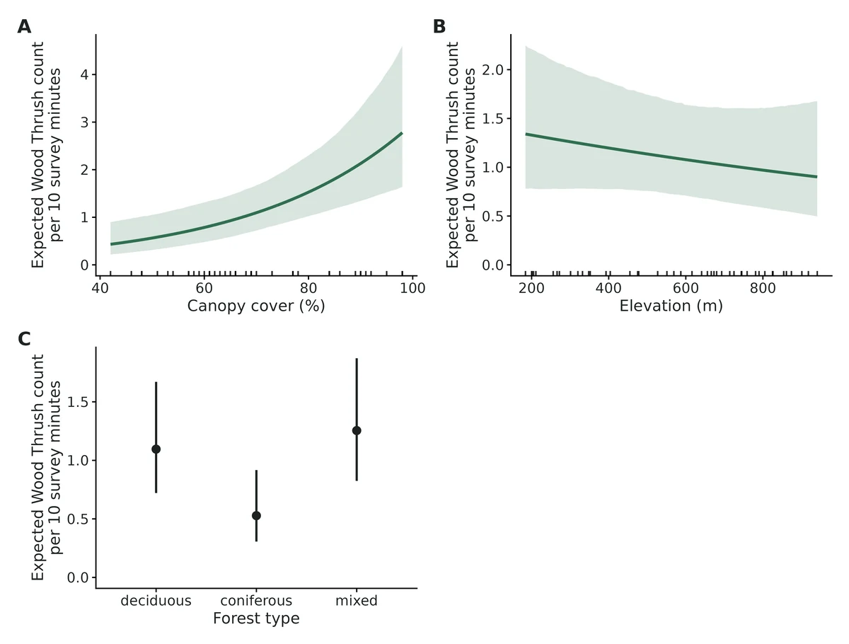
What this means
- Per 10 percentage points of canopy cover (%) this is associated with a 39% higher expected Wood Thrush count (rate ratio 1.39, 95% CI 1.18 to 1.64).
- Across the observed range of canopy cover (%) (42 to 98), with other continuous predictors at their mean; forest type = deciduous; typical station, the expected Wood Thrush count goes from 0.432 to 2.78.
- Per 100 m of elevation (m) this is associated with a 5.1% lower expected Wood Thrush count (rate ratio 0.949, 95% CI 0.854 to 1.05). The 95% interval includes no effect: the data are compatible with effects from 31% lower to 13% higher, including none.
- Compared with forest type = deciduous (reference), forest type = conifer is associated with a 52% lower expected Wood Thrush count (rate ratio 0.482, 95% CI 0.248 to 0.935): 0.528 vs 1.1.
- Compared with forest type = deciduous (reference), forest type = mixed is associated with a 15% higher expected Wood Thrush count (rate ratio 1.15, 95% CI 0.651 to 2.01): 1.25 vs 1.1. The 95% interval includes no effect: the data are compatible with effects from 35% lower to 101% higher, including none.
- Model checks: DHARMa simulated residuals showed no detectable problems with distribution, dispersion, outliers or zeros (all p >= 0.05).
- These are effects on the expected count as recorded, which combines how many/whether animals are present with how likely they are to be detected or recorded.
More figures
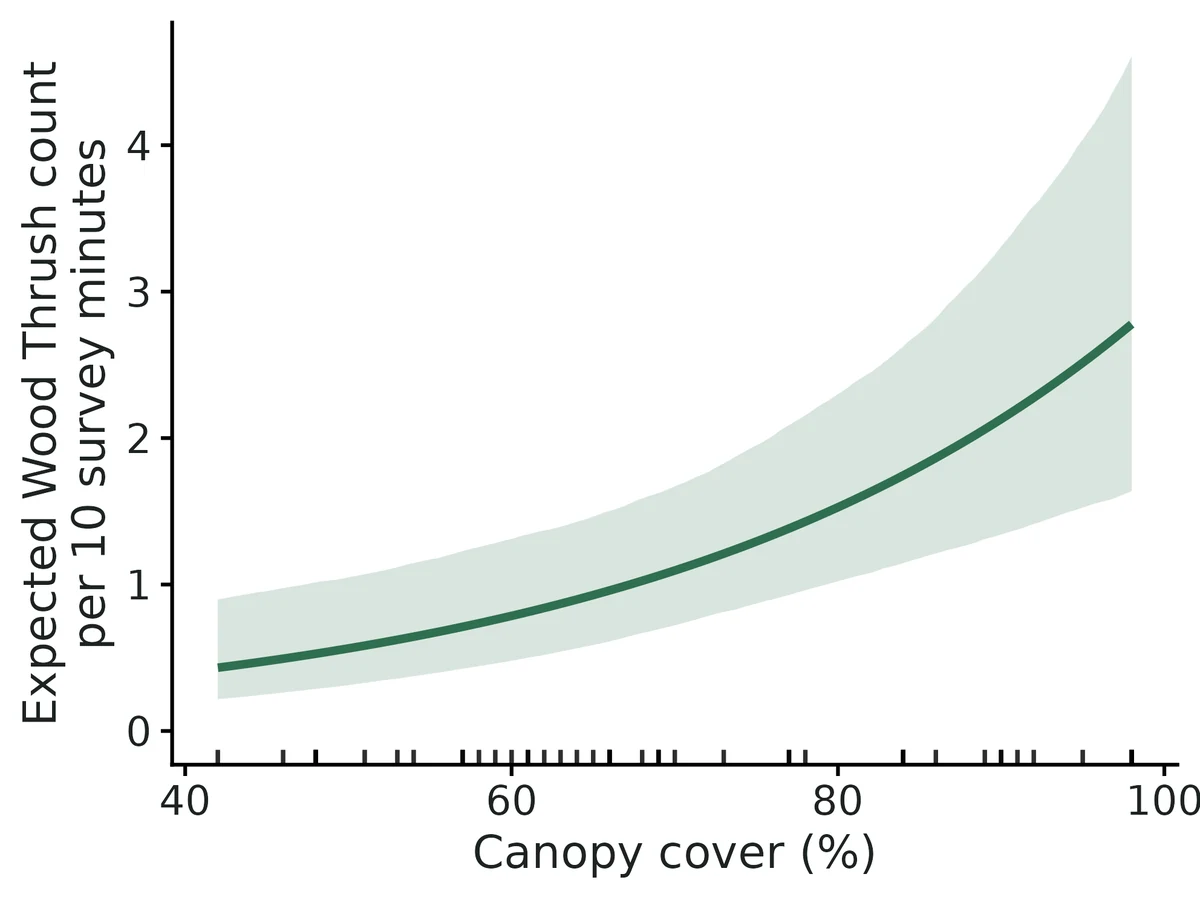
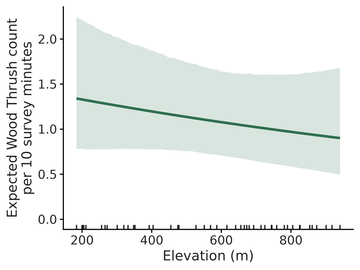
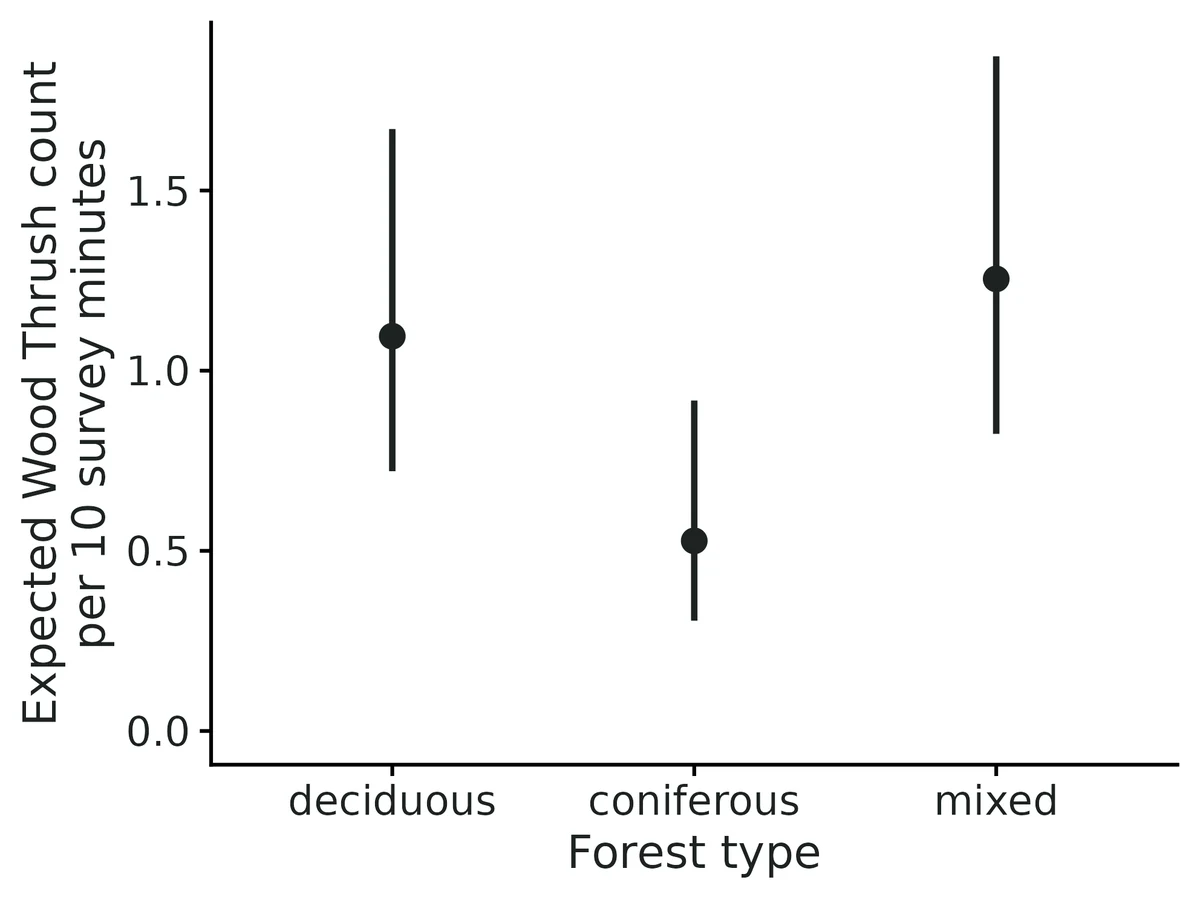
Figures are the module's default publication figures, reduced for the web. The report also saves them as PDF and full-resolution PNG.
Planted truth at the example's design
Before trusting the example's results, the module was run on many simulated data sets with the same design and known true values. Each row is one quantity: did the method get it back? (What the thresholds are.)
All interpreted estimands (canopy, elevation, forest-type effects, mean count) pass planted truth at this design (|rel. bias| <= 7.2%, coverage 0.905-0.940); fit converged; DHARMa all p > 0.5; module cross-checked and negative controls in VALIDATION.md. Station SD (FAIL, -17.6% bias, 23% singular fits) and NB theta (unbounded in 7/199) are nuisance parameters and are not interpreted.
| This example | 45 bird-count stations, 4 visits each (180 counts) |
|---|---|
| Design the module was validated at | 30 sites, 8 visits each (240 counts), negative binomial mixed model |
The example has more stations (45 vs 30) but only half the visits per station, so fewer counts in total than the validated default. At 45 x 4 the effects that are interpreted passed (bias within 7.2%, coverage, meaning how often the 95% interval contained the truth, 0.905-0.940), but the between-station spread was biased -17.6% with 23% of simulated fits singular, so it is not interpreted. VALIDATION.md found the module breaks down at 10 sites x 4 visits (coverage 0.875-0.88 for site-level effects, station SD -42%).
These calls sit close to the pass/fail line. With another 199 simulated data sets they could come out the other way, so read them as “about at the limit” rather than as a clear pass or fail.
- beta_elevation_m (✓ PASS): coverage 0.905 against a minimum of 0.904.
- beta_intercept (✓ PASS): coverage 0.915 against a minimum of 0.904.
- mean_response_at_reference (✓ PASS): coverage 0.915 against a minimum of 0.904.
- rate_ratio_elevation_m (✓ PASS): coverage 0.905 against a minimum of 0.904.
10 of 12 rows pass; 4 are borderline.
| Quantity | True value | Average estimate | Bias | Allowed bias | Coverage (needed) | Result |
|---|---|---|---|---|---|---|
| beta_canopy_cover_pct | 0.39 | 0.387 | -0.9% | ±10.0% | 0.94 (0.904) | ✓ PASS |
| beta_elevation_m | -0.28 | -0.275 | +1.8% | ±10.7%† | 0.91 (0.904) | ✓ PASS ≈ borderline |
| beta_forest_type_conifer | -0.9 | -0.89 | +1.1% | ±10.0% | 0.94 (0.904) | ✓ PASS |
| beta_forest_type_mixed | -0.25 | -0.245 | +2.0% | ±25.1%† | 0.93 (0.904) | ✓ PASS |
| beta_intercept | -2.08 | -2.1 | -1.0% | ±10.0% | 0.92 (0.904) | ✓ PASS ≈ borderline |
| mean_response_at_reference | 0.125 | 0.125 | +0.2% | ±10.0% | 0.92 (0.904) | ✓ PASS ≈ borderline |
| nb_size_theta | 3 | – | – | ±1916038694.7%† | – (0.904) | ✗ FAIL |
| rate_ratio_canopy_cover_pct | 1.48 | 1.48 | +0.5% | ±10.0% | 0.94 (0.904) | ✓ PASS |
| rate_ratio_elevation_m | 0.756 | 0.767 | +1.5% | ±10.0% | 0.91 (0.904) | ✓ PASS ≈ borderline |
| rate_ratio_forest_type_conifer | 0.407 | 0.436 | +7.2% | ±10.0% | 0.94 (0.904) | ✓ PASS |
| rate_ratio_forest_type_mixed | 0.779 | 0.817 | +4.9% | ±10.0% | 0.93 (0.904) | ✓ PASS |
| re_sd_station | 0.45 | 0.371 | -17.6% | ±11.1%† | 0.94 (0.904) | ✗ FAIL |
Limits that matter
- At 45 stations x 4 visits with ~1 bird per count, the station random-intercept SD is biased -18% (23% of simulated fits singular) and NB theta is sometimes unbounded: neither is interpreted (this run).
- Rate ratios for imprecise contrasts are biased upward in the mean (exp of a noisy log ratio): +7.2% conifer, +4.9% mixed here; log-scale coefficients unbiased (Known limit 1).
- Wald intervals only; recovery coverage 0.905-0.940 at this design (Known limit 4).
- Expected counts are for a typical station (random effect 0), not the landscape mean (Known limit 5).
- Counts confound abundance and detection; a canopy effect could partly be detectability (N-mixture module separates them).
- Spatial autocorrelation among stations is not modelled (Known limit 7).
- Associations, not causal effects.
All known limits from the module's validation record
- Odds/rate ratios for imprecise contrasts are biased upward in the mean. exp(beta-hat) is median-unbiased but not mean-unbiased: E[exp(b)] is about exp(beta + SE^2/2). When the SE of a log ratio exceeds about 0.35 (factor contrasts in Bernoulli GLMMs; small samples), the ratio estimand fails the mean-bias gate: +13% (binomial_glmm habitat), +15-90% in the small designs. The link-scale coefficient passes and the ratio's 95% CI keeps nominal coverage. Report ratios with their CIs; do not average point ratios across studies.
- Few groups. With 10 sites x 4 visits (NB GLMM) Wald intervals for site-level effects under-cover (0.875-0.88) and the site SD is biased -42%. With 15 Bernoulli sites x 4 the site SD interval under-covers (0.845). The module flags fewer than 5 levels; between 5 and ~15 groups, treat site-level effects' intervals as somewhat optimistic and run a planted-truth check at the researcher's design. Power below ~20 sites is low for site-level effects in any case.
- NB size theta needs data. With 100 observations and 30% structural zeros, theta is biased +29% (coverage 0.87). Overdispersion is then hard to separate from zero inflation; the coefficients and zero-inflation probability are still recovered.
- Wald intervals. All intervals are Wald (log scale for SDs and dispersion). Profile or bootstrap intervals are not implemented. For random-effect SDs near zero the interval is meaningless and the report says the fit is singular.
mean_response_at_referenceis for a typical group (random effect = 0), not the population average.- Not validated: random slopes (rejected by the parser), non-default links (probit, cloglog, inverse; accepted but their interpretation sentences are generic), zero-inflation formulas other than
~1(supported, zi_beta_* reported, not recovery-tested), polynomial terms (supported in fitting and plots, not recovery-tested), thestats::glmfallback engine (cross-checked to agree, not separately recovery-tested), and DHARMa test calibration (the tests come from DHARMa, unmodified). - Spatial/temporal autocorrelation is not modelled or tested for.
How this module was validated
- 200 simulated data sets per design (500 for false-positive checks), fitted with glmmTMB using REML for mixed models; all 200 converged at the default design and every one of 12 quantities passed.
- Nine model families (Gaussian, binomial, Poisson, beta, Gamma, zero-inflated and interaction models) each tested with 200 replicates; all passed except odds ratios for factor contrasts in the binary mixed model (+13% mean bias, a known back-transformation effect).
- Harder small designs failed as expected: 10 sites x 4 visits (coverage 0.875-0.88, site SD -42%), 15 binary sites x 4 visits, and a small zero-inflated design (theta +29%).
- Negative controls: with no true effect, intervals excluded zero 5.8% and 4.2% of the time (nominal 5%); fitting Poisson to overdispersed data or dropping the site random effect failed the gate, as it should.
- Cross-checked on 20 data sets per case against lme4, stats::glm, MASS::glm.nb and hand-written likelihoods; coefficients agreed to within 0.14 standard errors at most.
- Power: about 40 sites give 80% power for a site-level effect of 0.3 per SD (power 0.74 at 30 sites, 0.93 at 50).
- A separate verifier agent reran the builder's runs exactly, passed three new designs with its own simulators, confirmed the controls fail, and fixed an offset-matching bug and several report-wording issues.
Every run uses the acceptance gate described on the validation page. The full record follows, section by section, exactly as kept in the module's VALIDATION.md.
Settings and pass/fail rule used for every run
Date: 2026-10-18. Code state: dev/glm/code_md5_final_suite.txt (all runs below). Later changes touch only plotting code in output.R and the engine description string in module.R (residual-panel subtitles, and a module-local grouped conditional-effects plot for interactions); recovery never calls it. Final hashes: dev/glm/code_md5_after_plot_tweak.txt. 2026-10-19: figures.R (publication figure suite, glm_figures) added and registered in module.R; it only reads the fit (no change to simulate/fit/estimates), so the results below still apply. Dev tests: dev/glm/figs/test_figs.R. Engine: glmmTMB 1.1.15.2, R 4.5.3. Gate: recovery_gate() with its fixed thresholds (|bias| <= max(10% of truth, 3 MC SE); coverage >= 0.95 - 3 MC SE, here 0.904 for 200 reps and 0.921 for 500; >= 90% converged). Recovery uses fast_settings (identical to the real-data settings except no DHARMa/R2), REML for mixed models.
Reproduce: bash dev/glm/run_validation.sh (configs in modules/glm/validation/; outputs in results/glm/validation/<run>/), bin/Rscript dev/glm/crosscheck.R, bin/Rscript dev/glm/nb_ll_check.R. Tables below come from dev/glm/validation_tables.R. Each fit takes 0.3-0.9 s, so all 3,700 recovery fits took about 25 min on 16 cores.
1. Default design (nsim = 200): PASS on every estimand
NB2 GLMM, 30 sites x 8 visits, site-level forest cover (normal 55 +/- 20) and habitat (3 levels), visit-level temperature, effort offset U(0.5, 2), theta = 2, site SD = 0.5. 200/200 converged.
| estimand | truth | mean est | rel. bias % | bias MCSE | coverage | power | gate |
|---|---|---|---|---|---|---|---|
| beta_forest | 0.3 | 0.283 | -5.8 | 0.0084 | 0.955 | 0.645 | PASS |
| beta_habitat_riparian | 0.4 | 0.402 | 0.4 | 0.021 | 0.930 | 0.310 | PASS |
| beta_habitat_wetland | -0.3 | -0.267 | 10.9 | 0.019 | 0.945 | 0.170 | PASS |
| beta_intercept | 0.7 | 0.682 | -2.6 | 0.014 | 0.930 | - | PASS |
| beta_temp | -0.2 | -0.206 | -3.2 | 0.0046 | 0.965 | 0.885 | PASS |
| mean_response_at_reference | 2.01 | 2.02 | 0.1 | 0.028 | 0.930 | - | PASS |
| nb_size_theta | 2 | 2.05 | 2.5 | 0.028 | 0.965 | - | PASS |
| rate_ratio_forest | 1.35 | 1.34 | -1.0 | 0.011 | 0.955 | - | PASS |
| rate_ratio_habitat_riparian | 1.49 | 1.56 | 4.6 | 0.034 | 0.930 | - | PASS |
| rate_ratio_habitat_wetland | 0.741 | 0.795 | 7.3 | 0.016 | 0.945 | - | PASS |
| rate_ratio_temp | 0.819 | 0.815 | -0.4 | 0.0038 | 0.965 | - | PASS |
| re_sd_site | 0.5 | 0.499 | -0.3 | 0.0082 | 0.970 | - | PASS |
(beta_habitat_wetland: 10.9% relative bias but |bias| 0.033 < 3 MC SE = 0.057, so it is within Monte Carlo noise.)
2. Every family (nsim = 200 each)
Full tables are in the appendix. Designs: 30 groups x 8 obs unless noted.
| run | design | converged | gate |
|---|---|---|---|
| gaussian_lmm | Gaussian LMM, sigma 2, site SD 1 | 200/200 | PASS all 8 estimands (re_sd -0.8%, residual_sd +0.4%) |
| binomial_glmm | Bernoulli GLMM, 40 sites x 8, site SD 0.7 | 200/200 | PASS 9/11. FAIL (mean bias): odds_ratio_habitat_riparian +13.1%, odds_ratio_habitat_wetland +13.3%. The link-scale contrasts PASS (+8.1%, +10.7%, within 3 MC SE) and their coverage is 0.945/0.970; see Known limits 1 |
| binomial_trials_glm | successes/trials (2-6), 120 units, no RE | 200/200 | PASS all 10 |
| poisson_glm | Poisson + offset, 150 units, no RE | 200/200 | PASS all 10 |
| beta_glmm | beta, phi 15, site SD 0.3 | 200/200 | PASS all 12 |
| gamma_glmm | Gamma (log), CV 0.4, site SD 0.3 | 200/200 | PASS all 12 |
| zip_glmm | ZIP GLMM, 20% structural zeros | 200/200 | PASS all 12 |
| zinb_glmm | ZINB GLMM, 20% zeros, theta 2 | 200/200 | PASS all 13 |
| interaction_glmm | Poisson GLMM + forest:temp + temp:habitat (one interaction truly 0) | 200/200 | PASS all 17 |
3. Harder designs (nsim = 200): where the module stops working
| run | design | result |
|---|---|---|
| hard_nb_small | NB GLMM with only 10 sites x 4 visits (40 obs) | FAIL. Coverage 0.875-0.88 for site-level effects (forest, wetland), intercept and mean response; re_sd_site biased -42%; rate_ratio_habitat_riparian +17% mean bias. Visit-level temp still PASSES (coverage 0.945). |
| hard_binomial_small | Bernoulli GLMM, 15 sites x 4 visits (60 obs) | Link-scale coefficients all PASS (coverage 0.965-0.98). FAIL: odds_ratio_forest mean bias +15.5% (retransformation); re_sd_site coverage 0.845. Power for any effect <= 0.17. |
| hard_zinb_small | ZINB, 100 obs, no RE, 30% zeros, theta 1 | All coefficients and zero_inflation_prob PASS. FAIL: nb_size_theta +29% bias, coverage 0.87. |
4. Negative controls: the gate can fail, and false positives are at the nominal rate
False-positive rate (effect = 0), nsim = 500 (null_effects: forest and temp effects 0, default design otherwise):
| estimand | rejection rate (95% CI excludes 0) | MC SE | coverage |
|---|---|---|---|
| beta_forest (site-level) | 0.058 | 0.010 | 0.942 |
| beta_temp (visit-level) | 0.042 | 0.009 | 0.958 |
Both are consistent with 0.05. For comparison, with ML instead of REML the site-level rate was 0.084 (coverage 0.916; results/glm/validation_ml/null_effects), which is why REML is the default for mixed models.
Mis-specified fits must fail the gate:
| run | mis-specification | outcome |
|---|---|---|
| misspec_poisson | NB data (theta 2) fitted as Poisson GLMM | FAIL as expected: beta_temp coverage 0.680 (bound 0.904), re_sd_site +14% bias / coverage 0.845 |
| misspec_norandom | site random effect dropped (pseudoreplication of site-level covariates) | FAIL as expected: coverage beta_forest 0.715, riparian 0.685, wetland 0.760, intercept 0.695; nb_size_theta -29% bias, coverage 0.39 |
5. Cross-check against independent implementations
dev/glm/crosscheck.R: 20 simulated datasets per case. The module's estimates are compared with lme4 (lmer, glmer, glmer.nb), stats::glm, MASS::glm.nb, and, where no package was available, hand-written likelihoods maximised with optim (beta, ZIP and ZINB GLMs; betareg/pscl are not installed). GLMM comparisons use the module with REML: false because glmer is ML only. Output: results/glm/validation/crosscheck_summary.csv.
| case | independent route | max \ | coef diff\ | / SE | max SE rel. diff | max dispersion/SD rel. diff |
|---|---|---|---|---|---|---|
| gaussian LMM, REML | lmer(REML = TRUE) | 1.0e-6 | 0.9% | 3.3e-6 | ||
| gaussian LMM, ML | lmer(REML = FALSE) | 5.2e-5 | 1.1% | 6.6e-6 | ||
| Bernoulli GLMM | glmer (Laplace) | 0.0033 | 1.1% | 8.6e-4 | ||
| Poisson GLMM | glmer | 0.00098 | 0.7% | 1.2e-4 | ||
| NB2 GLMM | glmer.nb | 0.143 | 6.7% | 1.2% | ||
| NB2 GLM | MASS::glm.nb | 0.00017 | 6.5% | 1.9e-5 | ||
| binomial trials GLM | glm | 6.4e-5 | 2.4e-6 | - | ||
| Gamma GLM | glm (coefs) + MASS::gamma.shape (ML shape) | 0.00014 | 6.1% | 8.1e-6 | ||
| beta GLM | hand-written likelihood | 9.6e-5 | 2.4e-6 | 4.6e-6 | ||
| ZIP GLM | hand-written likelihood | 1.2e-4 | 5.0e-6 | 1.3e-5 (zero-inflation prob.) | ||
| ZINB GLM | hand-written likelihood | 1.3e-4 | 1.3e-5 | 2.5e-5 |
Explained differences:
- SE differences of about 6% for glm.nb and glm(Gamma) arise because glm uses expected information and, for Gamma, the Pearson dispersion. glmmTMB uses the observed Hessian at the ML shape.
- NB2 GLMM vs glmer.nb: coefficients differ by up to 0.14 SE (median 0.11 SE). In
dev/glm/nb_ll_check.Rthe glmmTMB objective at the glmmTMB MLE is higher than at glmer.nb's estimates in all 20 datasets, by 0.006 to 0.024 log-likelihood units (results/glm/validation/nb_glmm_loglik_check.csv). The module therefore reaches the better optimum. glmer.nb's own reported log-likelihood differs from glmmTMB's by -0.06 to +0.12, so the two packages evaluate this likelihood differently; glmer.nb fits theta in an outer loop. The difference is small next to the SEs.
6. Power over a design knob (nsim = 100 per point)
core/run.R power glm --vary n_groups=10,20,30,50,80 --nsim 100 (default design, 8 visits per site; results/glm/validation/power_ngroups/).
| sites | power: forest (site-level, 0.3/SD) | power: temp (visit-level, -0.2/SD) | power: riparian vs upland (0.4) | coverage forest | re_sd rel. bias |
|---|---|---|---|---|---|
| 10 | 0.34 | 0.32 | 0.19 | 0.88 | -16% |
| 20 | 0.53 | 0.69 | 0.29 | 0.94 | -2% |
| 30 | 0.74 | 0.86 | 0.45 | 0.95 | -6% |
| 50 | 0.93 | 0.97 | 0.53 | 0.96 | -2% |
| 80 | 1.00 | 1.00 | 0.68 | 0.95 | -1% |
About 40 sites give 80% power for a site-level effect of 0.3 per SD (rate ratio 1.35); a 3-level habitat contrast of 0.4 needs more than 80 sites. At 10 sites coverage is below nominal (0.88), consistent with hard_nb_small.
7. Example data (real-data format) and reports
bin/Rscript core/run.R fit glm --config modules/glm/example/config.yaml --out results/glm/example (plus config_binomial.yaml, config_beta.yaml). The examples were simulated with known values (dev/glm/make_examples.R, dev/glm/example_truth.txt). All three converged, DHARMa tests all p > 0.4, and every generating value is inside its 95% CI:
- Wood Thrush NB2 GLMM: canopy rate ratio per 10 points 1.38 (1.17-1.62), truth exp(0.25) = 1.28; conifer vs deciduous 0.50 (0.26-0.96), truth 0.41; elevation per 100 m 0.95 (0.86-1.06), truth 0.89; station SD 0.56 (0.34-0.93), truth 0.45.
- Hatching binomial GLMM: OR per 1 m nest height 1.28 (1.09-1.50), truth 1.28; per 50 m from edge 1.65 (1.30-2.09), truth 1.49; predator guard 1.87 (1.17-3.0), truth 2.01.
- Seagrass beta GLMM: OR per 1 m depth 0.645 (0.576-0.721), truth 0.638; per 5 NTU 0.727 (0.60-0.88), truth 0.741; phi 12.1 (8.8-16.6), truth 12.
I read the HTML reports. The interpretation sentences match the estimates table: rate ratios, percentage changes, response-scale predictions across observed ranges, the random-effect spread and the dispersion statements. Conditional-effect plots render on the response scale with 95% bands and rugs. Factors are drawn as points with intervals, and interactions as several coloured curves with bands (dev/glm/inter_png.R; the core cond_effect_plot() loses its grouping under ggplot2 4.0, so the module draws grouped curves itself). The forest plot and DHARMa panels render as well.
ML vs REML (why REML is the default for mixed models)
An earlier full suite used ML (results/glm/validation_ml/, same configs). Under ML, re_sd_site was biased low in every mixed design: -11.9% default, -11.6% Gaussian, -17.9% Bernoulli, -9.6% beta, -8.3% Gamma, -10.1% ZIP, -17.3% ZINB. Group-level contrasts were under-covered in the ZIP/ZINB GLMMs (0.880-0.890 < 0.904), and the null false-positive rate for the site-level covariate was 0.084. Under REML (started from the ML solution) all of these pass: re_sd within +/-3%, ZI coverage 0.915-0.95, false-positive rate 0.058. With glmmTMB's default start, REML stopped at a spurious zero-SD optimum in 7/200 beta GLMM datasets. Restarting from the ML estimates reached a better REML optimum (lower objective, positive-definite Hessian) in all 7, so the module always starts REML from ML. If REML still fails to converge, the ML fit is reported with a note.
Independent verification (2026-10-18, separate verifier agent)
Scripts: dev/glm/verify/ (verify_recovery.R = own simulators + driver, run_verify.sh, rerun_after_fix.sh, usability.sh, messy/). Outputs: results/glm/verify/. Log: logs/glm_verify.log. Final code hashes: dev/glm/verify/code_md5_verified.txt.
Literature / parameterisation check. Engine assumptions were checked against glmmTMB 1.1.15.2 ?sigma.glmmTMB and Brooks et al. (2017): NB2 Var = mu(1 + mu/theta) with betadisp = log(theta); beta Var = mu(1-mu)/(1+phi) (Ferrari & Cribari-Neto 2004); Gamma sigma = 1/sqrt(shape) = CV, so the module's log CV = -0.5 x betadisp is right; zero inflation is a logit-link mixture with E[y] = (1-pi) mu. The module's simulator shares canon_family, link_inv and coef_label with the fitter and standardises with the sample SD exactly as the fitter does, so I did not reuse it.
Independent planted truth. My simulators (no module code) set truth on the RAW covariate scale and derive the per-SD estimands analytically (beta_SD = beta_raw x sample SD; intercept at the sample mean; for x:factor interactions, factor contrast = b2 + b3 x mean(x)). The per-unit estimands (*_per_<u>) are therefore checked against raw-scale truth that does not depend on the scaling code. Fitted with module$fit() + fast_settings; summarised with core summarise_recovery() / recovery_gate() (thresholds unchanged). All replicates converged.
| design (seed 777000+r) | nsim | result | ||
|---|---|---|---|---|
| Gamma GLMM, 40 ponds x 6, depth U(0.5,4) obs-level (-0.35/m), 2-level pond-level treatment (+0.25), CV 0.6, pond SD 0.4 | 200 | PASS 9/9. Max \ | rel. bias\ | 2.4% (mean response); coverage 0.93-0.96; ratio_of_means_depth_per_1 +0.5%, gamma_cv -0.7%, re_sd_pond -2.2% |
| Binomial successes/trials (1-10) GLMM, 25 colonies x 6, shrub (normal 30 +/- 12) x grazed interaction, colony SD 0.6 | 200 | PASS 10/10. Interaction coefficient +3.2%, odds_ratio_shrub_per_10 +0.2%, re_sd -0.2%; coverage 0.94-0.98 | ||
Zero-inflated Poisson GLM, n = 300, flow U(5,60), 3-level substrate, area offset reported per 10 quadrats (offset_per: 10), pi = 0.3 | 200 | PASS 10/10. Max \ | rel. bias\ | 0.7%; coverage 0.92-0.965; mean_response_at_reference (incl. zero inflation, per 10 units) -0.4% |
Controls (my designs).
- False-positive rate, Gamma design with both effects 0, nsim 500: obs-level depth 0.048, pond-level treatment 0.066 (MC SE 0.010). All 9 estimands PASS.
- ZIP data fitted as plain Poisson: FAIL as required (beta_intercept -43%, coverage 0.000; slopes coverage 0.745-0.815).
- Gamma GLMM fitted without the pond random effect: FAIL as required (pond-level treatment coverage 0.740, intercept 0.680, gamma_cv +15.5% / coverage 0.115). The obs-level depth effect still passes.
Builder's numbers reproduced. Rerunning recover for default (200), binomial_glmm (200) and null_effects (500) with the same seeds gave the tables in sections 1, 2 and 4 exactly (default PASS 12/12; binomial_glmm odds ratio FAILs +13.1% / +13.3%; FPR 0.058 / 0.042). After my engine fix (below), default, poisson_glm and gamma_glmm summaries are byte-identical to the builder's (results/glm/verify/after_fix/).
Problems found and fixed (module files only; core untouched).
- Offset partial matching (engine.R, module.R).
sp$offsetused R's partial$matching: if the spec had nooffsetelement but hadoffset_per, the value ofoffset_per(e.g. 1 or 10) was taken as the offset column, solog(df[[1]])(often the response) entered as an offset. In my first smoke test this made every Gamma GLMM fit collapse (slopes 0, CV 1e-7) and every binomial-trials fit fail. Throughread_data()the same happened when a config hadoffset_per:withoutoffset:(stopped with a confusing "column(s) 10 not found"). Now exact[["offset"]]lookups, plus a clearcheck_datamessage foroffset_perwithoutoffset. The builder's suite was not affected (its simulator always setsoffset). - Misspelled group ids (module.R).
WT03vsWT-03was silently fitted as a 46th station.check_datanow stops with "grouping column station has labels that look like the same station spelled differently: 'WT-03' (3 rows) vs 'WT03' (1 rows) ..." (case, punctuation and leading zeros ignored).fitnotes also flag single-observation groups when the typical group has >= 3. - Figure export (output.R). The figure named "Effect of canopy cover (%)" failed to save in core
export_figures()(%in the file name; ggsave treats it as a format string). The figure list names now spell out%and/. The underlying core issue (file stem = figure name, unsanitised) remains for other modules. - Interaction sentences (output.R). They read "Each 1-SD increase (or, for a factor, the named level instead of the reference) in forest_type_conifer multiplies the rate ratio for canopy_cover_pct by 0.922", with raw column names. Now: "when forest type = conifer rather than deciduous, the rate ratio per 1 SD of canopy cover (%) (15.6) is multiplied by 0.922 (95% CI 0.49 to 1.74)". Identity-link and continuous x continuous versions were checked too.
- Detection caveat (output.R). For count and 0/1 families the interpretation now says that effects on recorded counts/detections combine abundance/occurrence with detectability, and points to occupancy / N-mixture modules. Not added for successes/trials, beta, Gamma or gaussian.
- Missing-value message now says "data rows N, not counting the header line".
Usability. On the Wood Thrush example every sentence was checked by hand against the estimates table (for example RR per 10 points = exp(0.500 x 10/15.6) = 1.378; station spread exp(+/-1.96 x 0.56) = 0.334-3.0; NB variance/mean at the mean count 1 + 1.13/5.89 = 1.19; conifer 1.156 x 0.498 = 0.576). The canopy curve (0.47 to 2.84) and forest-type points (1.16 / 0.576 / 1.32) match. Wording is associational and states that the response is a count per 10 minutes. The NA, wrong-column-name (lists the columns present, explains canopy cover pct became canopy.cover.pct), typo and offset_per messages are actionable. Binomial and beta example sentences were checked the same way.
Not fixed / still open. The module has no figures(fit, data, opts) per the newer MODULE_SPEC / FIGURES.md; core falls back to plots(). Core's journal styling moves the interaction legend to the right, which squeezes the panel. Core export_figures() does not sanitise file names. The known limits above (ratio retransformation bias, few groups, theta with 100 obs) are confirmed, not changed.
Appendix: full recovery tables (REML suite)
default: 200 replicates, 200 converged (100.0%), 0 errors, coverage bound 0.904; mean fit time 0.87 s
| estimand | truth | mean est | rel. bias % | bias MCSE | coverage | power | gate |
|---|---|---|---|---|---|---|---|
| beta_forest | 0.3 | 0.283 | -5.8 | 0.0084 | 0.955 | 0.645 | PASS |
| beta_habitat_riparian | 0.4 | 0.402 | 0.4 | 0.021 | 0.930 | 0.310 | PASS |
| beta_habitat_wetland | -0.3 | -0.267 | 10.9 | 0.019 | 0.945 | 0.170 | PASS |
| beta_intercept | 0.7 | 0.682 | -2.6 | 0.014 | 0.930 | - | PASS |
| beta_temp | -0.2 | -0.206 | -3.2 | 0.0046 | 0.965 | 0.885 | PASS |
| mean_response_at_reference | 2.01 | 2.02 | 0.1 | 0.028 | 0.930 | - | PASS |
| nb_size_theta | 2 | 2.05 | 2.5 | 0.028 | 0.965 | - | PASS |
| rate_ratio_forest | 1.35 | 1.34 | -1.0 | 0.011 | 0.955 | - | PASS |
| rate_ratio_habitat_riparian | 1.49 | 1.56 | 4.6 | 0.034 | 0.930 | - | PASS |
| rate_ratio_habitat_wetland | 0.741 | 0.795 | 7.3 | 0.016 | 0.945 | - | PASS |
| rate_ratio_temp | 0.819 | 0.815 | -0.4 | 0.0038 | 0.965 | - | PASS |
| re_sd_site | 0.5 | 0.499 | -0.3 | 0.0082 | 0.970 | - | PASS |
gaussian_lmm: 200 replicates, 200 converged (100.0%), 0 errors, coverage bound 0.904; mean fit time 0.53 s
| estimand | truth | mean est | rel. bias % | bias MCSE | coverage | power | gate |
|---|---|---|---|---|---|---|---|
| beta_forest | 1 | 0.967 | -3.3 | 0.015 | 0.950 | 0.990 | PASS |
| beta_habitat_riparian | 0.8 | 0.832 | 4.0 | 0.04 | 0.935 | 0.300 | PASS |
| beta_habitat_wetland | -0.6 | -0.528 | 11.9 | 0.038 | 0.950 | 0.170 | PASS |
| beta_intercept | 10 | 9.96 | -0.4 | 0.027 | 0.950 | - | PASS |
| beta_temp | -0.5 | -0.494 | 1.2 | 0.0097 | 0.925 | 0.955 | PASS |
| mean_response_at_reference | 10 | 9.96 | -0.4 | 0.027 | 0.950 | - | PASS |
| re_sd_site | 1 | 0.992 | -0.8 | 0.014 | 0.975 | - | PASS |
| residual_sd | 2 | 2.01 | 0.4 | 0.0072 | 0.930 | - | PASS |
binomial_glmm: 200 replicates, 200 converged (100.0%), 0 errors, coverage bound 0.904; mean fit time 0.57 s
| estimand | truth | mean est | rel. bias % | bias MCSE | coverage | power | gate |
|---|---|---|---|---|---|---|---|
| beta_forest | 0.4 | 0.397 | -0.8 | 0.011 | 0.970 | 0.585 | PASS |
| beta_habitat_riparian | 0.5 | 0.541 | 8.1 | 0.029 | 0.945 | 0.240 | PASS |
| beta_habitat_wetland | -0.4 | -0.357 | 10.7 | 0.028 | 0.970 | 0.135 | PASS |
| beta_intercept | -0.5 | -0.494 | 1.3 | 0.019 | 0.970 | - | PASS |
| beta_temp | -0.3 | -0.3 | 0.1 | 0.0083 | 0.980 | 0.650 | PASS |
| mean_response_at_reference | 0.378 | 0.381 | 1.0 | 0.0044 | 0.970 | - | PASS |
| odds_ratio_forest | 1.49 | 1.5 | 0.8 | 0.017 | 0.970 | - | PASS |
| odds_ratio_habitat_riparian | 1.65 | 1.87 | 13.1 | 0.058 | 0.945 | - | FAIL (bias) |
| odds_ratio_habitat_wetland | 0.67 | 0.759 | 13.3 | 0.023 | 0.970 | - | FAIL (bias) |
| odds_ratio_temp | 0.741 | 0.746 | 0.7 | 0.006 | 0.980 | - | PASS |
| re_sd_site | 0.7 | 0.692 | -1.2 | 0.018 | 0.945 | - | PASS |
binomial_trials_glm: 200 replicates, 200 converged (100.0%), 0 errors, coverage bound 0.904; mean fit time 0.32 s
| estimand | truth | mean est | rel. bias % | bias MCSE | coverage | power | gate |
|---|---|---|---|---|---|---|---|
| beta_forest | 0.4 | 0.397 | -0.7 | 0.0054 | 0.960 | 1.000 | PASS |
| beta_habitat_riparian | 0.5 | 0.471 | -5.9 | 0.014 | 0.940 | 0.690 | PASS |
| beta_habitat_wetland | -0.4 | -0.427 | -6.7 | 0.012 | 0.970 | 0.660 | PASS |
| beta_intercept | 0.3 | 0.325 | 8.2 | 0.0091 | 0.945 | - | PASS |
| beta_temp | -0.3 | -0.301 | -0.3 | 0.005 | 0.960 | 0.985 | PASS |
| mean_response_at_reference | 0.574 | 0.58 | 1.0 | 0.0022 | 0.945 | - | PASS |
| odds_ratio_forest | 1.49 | 1.49 | 0.0 | 0.0082 | 0.960 | - | PASS |
| odds_ratio_habitat_riparian | 1.65 | 1.63 | -1.1 | 0.022 | 0.940 | - | PASS |
| odds_ratio_habitat_wetland | 0.67 | 0.662 | -1.3 | 0.0078 | 0.970 | - | PASS |
| odds_ratio_temp | 0.741 | 0.742 | 0.2 | 0.0037 | 0.960 | - | PASS |
poisson_glm: 200 replicates, 200 converged (100.0%), 0 errors, coverage bound 0.904; mean fit time 0.34 s
| estimand | truth | mean est | rel. bias % | bias MCSE | coverage | power | gate |
|---|---|---|---|---|---|---|---|
| beta_forest | 0.3 | 0.293 | -2.3 | 0.003 | 0.970 | 1.000 | PASS |
| beta_habitat_riparian | 0.4 | 0.387 | -3.2 | 0.0069 | 0.975 | 0.980 | PASS |
| beta_habitat_wetland | -0.3 | -0.307 | -2.4 | 0.0079 | 0.950 | 0.800 | PASS |
| beta_intercept | 0.7 | 0.707 | 1.0 | 0.0053 | 0.960 | - | PASS |
| beta_temp | -0.2 | -0.2 | 0.1 | 0.0031 | 0.950 | 0.985 | PASS |
| mean_response_at_reference | 2.01 | 2.03 | 1.0 | 0.011 | 0.960 | - | PASS |
| rate_ratio_forest | 1.35 | 1.34 | -0.6 | 0.004 | 0.970 | - | PASS |
| rate_ratio_habitat_riparian | 1.49 | 1.48 | -0.8 | 0.01 | 0.975 | - | PASS |
| rate_ratio_habitat_wetland | 0.741 | 0.74 | -0.1 | 0.0059 | 0.950 | - | PASS |
| rate_ratio_temp | 0.819 | 0.82 | 0.1 | 0.0026 | 0.950 | - | PASS |
beta_glmm: 200 replicates, 200 converged (100.0%), 0 errors, coverage bound 0.904; mean fit time 0.91 s
| estimand | truth | mean est | rel. bias % | bias MCSE | coverage | power | gate |
|---|---|---|---|---|---|---|---|
| beta_forest | 0.3 | 0.291 | -3.1 | 0.0046 | 0.945 | 0.995 | PASS |
| beta_habitat_riparian | 0.3 | 0.31 | 3.4 | 0.011 | 0.945 | 0.465 | PASS |
| beta_habitat_wetland | -0.3 | -0.29 | 3.4 | 0.011 | 0.975 | 0.420 | PASS |
| beta_intercept | -0.5 | -0.502 | -0.4 | 0.008 | 0.945 | - | PASS |
| beta_precision_phi | 15 | 15.1 | 0.4 | 0.099 | 0.955 | - | PASS |
| beta_temp | -0.2 | -0.199 | 0.6 | 0.0024 | 0.970 | 1.000 | PASS |
| mean_response_at_reference | 0.378 | 0.377 | -0.0 | 0.0019 | 0.945 | - | PASS |
| odds_ratio_forest | 1.35 | 1.34 | -0.7 | 0.0062 | 0.945 | - | PASS |
| odds_ratio_habitat_riparian | 1.35 | 1.38 | 2.2 | 0.015 | 0.945 | - | PASS |
| odds_ratio_habitat_wetland | 0.741 | 0.757 | 2.2 | 0.0079 | 0.975 | - | PASS |
| odds_ratio_temp | 0.819 | 0.82 | 0.2 | 0.002 | 0.970 | - | PASS |
| re_sd_site | 0.3 | 0.302 | 0.5 | 0.0042 | 0.955 | - | PASS |
gamma_glmm: 200 replicates, 200 converged (100.0%), 0 errors, coverage bound 0.904; mean fit time 0.65 s
| estimand | truth | mean est | rel. bias % | bias MCSE | coverage | power | gate |
|---|---|---|---|---|---|---|---|
| beta_forest | 0.2 | 0.194 | -2.9 | 0.0044 | 0.970 | 0.865 | PASS |
| beta_habitat_riparian | 0.25 | 0.262 | 5.0 | 0.011 | 0.925 | 0.385 | PASS |
| beta_habitat_wetland | -0.2 | -0.184 | 7.9 | 0.011 | 0.935 | 0.235 | PASS |
| beta_intercept | 3 | 2.98 | -0.5 | 0.0075 | 0.935 | - | PASS |
| beta_temp | -0.15 | -0.148 | 1.1 | 0.002 | 0.965 | 1.000 | PASS |
| gamma_cv | 0.4 | 0.398 | -0.5 | 0.0013 | 0.965 | - | PASS |
| mean_response_at_reference | 20.1 | 19.9 | -1.0 | 0.15 | 0.935 | - | PASS |
| ratio_of_means_forest | 1.22 | 1.22 | -0.4 | 0.0054 | 0.970 | - | PASS |
| ratio_of_means_habitat_riparian | 1.28 | 1.31 | 2.4 | 0.014 | 0.925 | - | PASS |
| ratio_of_means_habitat_wetland | 0.819 | 0.841 | 2.7 | 0.009 | 0.935 | - | PASS |
| ratio_of_means_temp | 0.861 | 0.863 | 0.2 | 0.0017 | 0.965 | - | PASS |
| re_sd_site | 0.3 | 0.301 | 0.4 | 0.0037 | 0.965 | - | PASS |
zip_glmm: 200 replicates, 200 converged (100.0%), 0 errors, coverage bound 0.904; mean fit time 0.61 s
| estimand | truth | mean est | rel. bias % | bias MCSE | coverage | power | gate |
|---|---|---|---|---|---|---|---|
| beta_forest | 0.3 | 0.293 | -2.4 | 0.0077 | 0.955 | 0.740 | PASS |
| beta_habitat_riparian | 0.4 | 0.404 | 1.1 | 0.02 | 0.915 | 0.360 | PASS |
| beta_habitat_wetland | -0.3 | -0.278 | 7.3 | 0.018 | 0.950 | 0.165 | PASS |
| beta_intercept | 0.7 | 0.702 | 0.3 | 0.013 | 0.965 | - | PASS |
| beta_temp | -0.2 | -0.201 | -0.6 | 0.0031 | 0.955 | 0.985 | PASS |
| mean_response_at_reference | 1.61 | 1.64 | 1.8 | 0.022 | 0.975 | - | PASS |
| rate_ratio_forest | 1.35 | 1.35 | -0.1 | 0.011 | 0.955 | - | PASS |
| rate_ratio_habitat_riparian | 1.49 | 1.56 | 4.4 | 0.031 | 0.915 | - | PASS |
| rate_ratio_habitat_wetland | 0.741 | 0.783 | 5.7 | 0.014 | 0.950 | - | PASS |
| rate_ratio_temp | 0.819 | 0.819 | -0.0 | 0.0026 | 0.955 | - | PASS |
| re_sd_site | 0.5 | 0.502 | 0.4 | 0.0063 | 0.980 | - | PASS |
| zero_inflation_prob | 0.2 | 0.2 | 0.1 | 0.0026 | 0.930 | - | PASS |
zinb_glmm: 200 replicates, 200 converged (100.0%), 0 errors, coverage bound 0.904; mean fit time 0.88 s
| estimand | truth | mean est | rel. bias % | bias MCSE | coverage | power | gate |
|---|---|---|---|---|---|---|---|
| beta_forest | 0.3 | 0.282 | -5.9 | 0.0093 | 0.935 | 0.595 | PASS |
| beta_habitat_riparian | 0.4 | 0.413 | 3.2 | 0.023 | 0.915 | 0.315 | PASS |
| beta_habitat_wetland | -0.3 | -0.258 | 13.9 | 0.022 | 0.930 | 0.145 | PASS |
| beta_intercept | 0.7 | 0.653 | -6.7 | 0.016 | 0.915 | - | PASS |
| beta_temp | -0.2 | -0.208 | -4.0 | 0.0058 | 0.945 | 0.740 | PASS |
| mean_response_at_reference | 1.61 | 1.59 | -1.2 | 0.025 | 0.925 | - | PASS |
| nb_size_theta | 2 | 2.13 | 6.7 | 0.062 | 0.955 | - | PASS |
| rate_ratio_forest | 1.35 | 1.34 | -0.9 | 0.013 | 0.935 | - | PASS |
| rate_ratio_habitat_riparian | 1.49 | 1.59 | 6.9 | 0.039 | 0.915 | - | PASS |
| rate_ratio_habitat_wetland | 0.741 | 0.81 | 9.4 | 0.018 | 0.930 | - | PASS |
| rate_ratio_temp | 0.819 | 0.815 | -0.5 | 0.0048 | 0.945 | - | PASS |
| re_sd_site | 0.5 | 0.485 | -2.9 | 0.0098 | 0.980 | - | PASS |
| zero_inflation_prob | 0.2 | 0.189 | -5.4 | 0.0041 | 0.955 | - | PASS |
interaction_glmm: 200 replicates, 200 converged (100.0%), 0 errors, coverage bound 0.904; mean fit time 0.62 s
| estimand | truth | mean est | rel. bias % | bias MCSE | coverage | power | gate |
|---|---|---|---|---|---|---|---|
| beta_forest | 0.3 | 0.289 | -3.7 | 0.0073 | 0.930 | 0.780 | PASS |
| beta_forest_x_temp | 0.2 | 0.205 | 2.4 | 0.0031 | 0.965 | - | PASS |
| beta_habitat_riparian | 0.4 | 0.414 | 3.4 | 0.018 | 0.935 | 0.360 | PASS |
| beta_habitat_wetland | -0.3 | -0.273 | 8.9 | 0.017 | 0.955 | 0.155 | PASS |
| beta_intercept | 0.7 | 0.697 | -0.5 | 0.013 | 0.945 | - | PASS |
| beta_temp | -0.2 | -0.206 | -2.9 | 0.005 | 0.940 | 0.850 | PASS |
| beta_temp_x_habitat_riparian | 0.3 | 0.308 | 2.7 | 0.0069 | 0.970 | - | PASS |
| beta_temp_x_habitat_wetland | 0 | -0.000992 | - | 0.008 | 0.955 | - | PASS |
| mean_response_at_reference | 2.01 | 2.04 | 1.2 | 0.025 | 0.945 | - | PASS |
| rate_ratio_forest | 1.35 | 1.34 | -0.6 | 0.01 | 0.930 | - | PASS |
| rate_ratio_forest_x_temp | 1.22 | 1.23 | 0.6 | 0.0038 | 0.965 | - | PASS |
| rate_ratio_habitat_riparian | 1.49 | 1.56 | 4.8 | 0.029 | 0.935 | - | PASS |
| rate_ratio_habitat_wetland | 0.741 | 0.784 | 5.9 | 0.014 | 0.955 | - | PASS |
| rate_ratio_temp | 0.819 | 0.816 | -0.3 | 0.0041 | 0.940 | - | PASS |
| rate_ratio_temp_x_habitat_riparian | 1.35 | 1.37 | 1.3 | 0.0094 | 0.970 | - | PASS |
| rate_ratio_temp_x_habitat_wetland | 1 | 1.01 | 0.5 | 0.0081 | 0.955 | - | PASS |
| re_sd_site | 0.5 | 0.505 | 1.1 | 0.006 | 0.960 | - | PASS |
hard_nb_small: 200 replicates, 200 converged (100.0%), 0 errors, coverage bound 0.904; mean fit time 0.56 s
| estimand | truth | mean est | rel. bias % | bias MCSE | coverage | power | gate |
|---|---|---|---|---|---|---|---|
| beta_forest | 0.3 | 0.302 | 0.6 | 0.02 | 0.880 | 0.315 | FAIL (coverage) |
| beta_habitat_riparian | 0.4 | 0.394 | -1.4 | 0.04 | 0.905 | 0.155 | PASS |
| beta_habitat_wetland | -0.3 | -0.284 | 5.3 | 0.046 | 0.875 | 0.140 | FAIL (coverage) |
| beta_intercept | 0.7 | 0.658 | -6.0 | 0.028 | 0.880 | - | FAIL (coverage) |
| beta_temp | -0.2 | -0.227 | -13.3 | 0.013 | 0.925 | 0.225 | PASS |
| mean_response_at_reference | 2.01 | 2.09 | 3.8 | 0.06 | 0.880 | - | FAIL (coverage) |
| nb_size_theta | 2 | 281000 | 14034737.9 | 280000 | 0.965 | - | PASS |
| rate_ratio_forest | 1.35 | 1.41 | 4.5 | 0.031 | 0.880 | - | FAIL (coverage) |
| rate_ratio_habitat_riparian | 1.49 | 1.75 | 17.0 | 0.077 | 0.905 | - | FAIL (bias) |
| rate_ratio_habitat_wetland | 0.741 | 0.967 | 30.6 | 0.08 | 0.875 | - | FAIL (coverage) |
| rate_ratio_temp | 0.819 | 0.811 | -1.0 | 0.01 | 0.925 | - | PASS |
| re_sd_site | 0.5 | 0.288 | -42.4 | 0.027 | 0.980 | - | FAIL (bias) |
hard_binomial_small: 200 replicates, 200 converged (100.0%), 0 errors, coverage bound 0.904; mean fit time 0.51 s
| estimand | truth | mean est | rel. bias % | bias MCSE | coverage | power | gate |
|---|---|---|---|---|---|---|---|
| beta_forest | 0.4 | 0.459 | 14.7 | 0.029 | 0.970 | 0.180 | PASS |
| beta_habitat_riparian | 0.5 | 0.529 | 5.7 | 0.067 | 0.960 | 0.075 | PASS |
| beta_habitat_wetland | -0.4 | -0.423 | -5.8 | 0.069 | 0.965 | 0.060 | PASS |
| beta_intercept | -0.5 | -0.516 | -3.1 | 0.051 | 0.950 | - | PASS |
| beta_temp | -0.3 | -0.351 | -16.9 | 0.025 | 0.960 | 0.140 | PASS |
| mean_response_at_reference | 0.378 | 0.387 | 2.5 | 0.01 | 0.950 | - | PASS |
| odds_ratio_forest | 1.49 | 1.72 | 15.5 | 0.053 | 0.970 | - | FAIL (bias) |
| odds_ratio_habitat_riparian | 1.65 | 3.22 | 95.2 | 0.72 | 0.960 | - | PASS |
| odds_ratio_habitat_wetland | 0.67 | 1.22 | 81.9 | 0.27 | 0.965 | - | PASS |
| odds_ratio_temp | 0.741 | 0.749 | 1.1 | 0.018 | 0.960 | - | PASS |
| re_sd_site | 0.7 | 0.759 | 8.4 | 0.066 | 0.845 | - | FAIL (coverage) |
hard_zinb_small: 200 replicates, 200 converged (100.0%), 0 errors, coverage bound 0.904; mean fit time 0.36 s
| estimand | truth | mean est | rel. bias % | bias MCSE | coverage | power | gate |
|---|---|---|---|---|---|---|---|
| beta_forest | 0.3 | 0.29 | -3.3 | 0.0079 | 0.925 | 0.795 | PASS |
| beta_habitat_riparian | 0.4 | 0.392 | -2.0 | 0.018 | 0.940 | 0.330 | PASS |
| beta_habitat_wetland | -0.3 | -0.298 | 0.5 | 0.019 | 0.950 | 0.205 | PASS |
| beta_intercept | 0.7 | 0.679 | -3.1 | 0.017 | 0.935 | - | PASS |
| beta_temp | -0.2 | -0.198 | 0.9 | 0.0086 | 0.920 | 0.475 | PASS |
| mean_response_at_reference | 1.41 | 1.4 | -0.9 | 0.02 | 0.935 | - | PASS |
| nb_size_theta | 1 | 1.29 | 29.1 | 0.039 | 0.870 | - | FAIL (bias, coverage) |
| rate_ratio_forest | 1.35 | 1.34 | -0.4 | 0.011 | 0.925 | - | PASS |
| rate_ratio_habitat_riparian | 1.49 | 1.53 | 2.6 | 0.029 | 0.940 | - | PASS |
| rate_ratio_habitat_wetland | 0.741 | 0.77 | 4.0 | 0.016 | 0.950 | - | PASS |
| rate_ratio_temp | 0.819 | 0.826 | 0.9 | 0.0072 | 0.920 | - | PASS |
| zero_inflation_prob | 0.3 | 0.3 | -0.1 | 0.0068 | 0.915 | - | PASS |
null_effects: 500 replicates, 500 converged (100.0%), 0 errors, coverage bound 0.921; mean fit time 0.67 s
| estimand | truth | mean est | rel. bias % | bias MCSE | coverage | power | gate |
|---|---|---|---|---|---|---|---|
| beta_forest | 0 | 7.81e-05 | - | 0.0053 | 0.942 | 0.058 | PASS |
| beta_habitat_riparian | 0.4 | 0.39 | -2.6 | 0.012 | 0.950 | 0.284 | PASS |
| beta_habitat_wetland | -0.3 | -0.282 | 6.1 | 0.012 | 0.952 | 0.164 | PASS |
| beta_intercept | 0.7 | 0.685 | -2.2 | 0.0087 | 0.954 | - | PASS |
| beta_temp | 0 | 0.000329 | - | 0.0028 | 0.958 | 0.042 | PASS |
| mean_response_at_reference | 2.01 | 2.02 | 0.4 | 0.018 | 0.954 | - | PASS |
| nb_size_theta | 2 | 2.04 | 2.0 | 0.018 | 0.938 | - | PASS |
| rate_ratio_forest | 1 | 1.01 | 0.7 | 0.0054 | 0.942 | - | PASS |
| rate_ratio_habitat_riparian | 1.49 | 1.53 | 2.8 | 0.019 | 0.950 | - | PASS |
| rate_ratio_habitat_wetland | 0.741 | 0.783 | 5.7 | 0.0098 | 0.952 | - | PASS |
| rate_ratio_temp | 1 | 1 | 0.2 | 0.0028 | 0.958 | - | PASS |
| re_sd_site | 0.5 | 0.49 | -1.9 | 0.0051 | 0.976 | - | PASS |
misspec_poisson: 200 replicates, 200 converged (100.0%), 0 errors, coverage bound 0.904; mean fit time 0.55 s
| estimand | truth | mean est | rel. bias % | bias MCSE | coverage | power | gate |
|---|---|---|---|---|---|---|---|
| beta_forest | 0.3 | 0.281 | -6.3 | 0.0084 | 0.950 | 0.645 | PASS |
| beta_habitat_riparian | 0.4 | 0.403 | 0.7 | 0.021 | 0.945 | 0.310 | PASS |
| beta_habitat_wetland | -0.3 | -0.264 | 11.8 | 0.02 | 0.940 | 0.150 | PASS |
| beta_intercept | 0.7 | 0.67 | -4.3 | 0.014 | 0.925 | - | PASS |
| beta_temp | -0.2 | -0.206 | -3.2 | 0.0053 | 0.680 | 0.960 | FAIL (coverage) |
| mean_response_at_reference | 2.01 | 1.99 | -1.0 | 0.028 | 0.925 | - | PASS |
| rate_ratio_forest | 1.35 | 1.33 | -1.2 | 0.011 | 0.950 | - | PASS |
| rate_ratio_habitat_riparian | 1.49 | 1.56 | 4.7 | 0.034 | 0.945 | - | PASS |
| rate_ratio_habitat_wetland | 0.741 | 0.798 | 7.7 | 0.016 | 0.940 | - | PASS |
| rate_ratio_temp | 0.819 | 0.816 | -0.4 | 0.0044 | 0.680 | - | FAIL (coverage) |
| re_sd_site | 0.5 | 0.572 | 14.3 | 0.007 | 0.845 | - | FAIL (bias, coverage) |
misspec_norandom: 200 replicates, 200 converged (100.0%), 0 errors, coverage bound 0.904; mean fit time 0.35 s
| estimand | truth | mean est | rel. bias % | bias MCSE | coverage | power | gate |
|---|---|---|---|---|---|---|---|
| beta_forest | 0.3 | 0.283 | -5.8 | 0.0088 | 0.715 | 0.880 | FAIL (coverage) |
| beta_habitat_riparian | 0.4 | 0.407 | 1.8 | 0.022 | 0.685 | 0.590 | FAIL (coverage) |
| beta_habitat_wetland | -0.3 | -0.273 | 8.9 | 0.02 | 0.760 | 0.410 | FAIL (coverage) |
| beta_intercept | 0.7 | 0.793 | 13.3 | 0.015 | 0.695 | - | FAIL (bias, coverage) |
| beta_temp | -0.2 | -0.21 | -4.8 | 0.005 | 0.945 | 0.850 | PASS |
| mean_response_at_reference | 2.01 | 2.26 | 12.2 | 0.034 | 0.695 | - | FAIL (bias, coverage) |
| nb_size_theta | 2 | 1.43 | -28.7 | 0.019 | 0.390 | - | FAIL (bias, coverage) |
| rate_ratio_forest | 1.35 | 1.34 | -1.0 | 0.012 | 0.715 | - | FAIL (coverage) |
| rate_ratio_habitat_riparian | 1.49 | 1.58 | 5.9 | 0.036 | 0.685 | - | FAIL (coverage) |
| rate_ratio_habitat_wetland | 0.741 | 0.794 | 7.1 | 0.017 | 0.760 | - | FAIL (coverage) |
| rate_ratio_temp | 0.819 | 0.813 | -0.7 | 0.0041 | 0.945 | - | PASS |
Engine, references and full details
Engine: glmmTMB (REML for models with random intercepts, ML otherwise; Laplace approximation); stats::glm / MASS::glm.nb fallback for fixed-effects-only models.
References
- Brooks ME, Kristensen K, van Benthem KJ, Magnusson A, Berg CW, Nielsen A, Skaug HJ, Maechler M, Bolker BM (2017). glmmTMB balances speed and flexibility among packages for zero-inflated generalized linear mixed modeling. The R Journal 9(2):378-400. doi:10.32614/RJ-2017-066
- Bolker BM, Brooks ME, Clark CJ, Geange SW, Poulsen JR, Stevens MHH, White J-SS (2009). Generalized linear mixed models: a practical guide for ecology and evolution. Trends in Ecology and Evolution 24(3):127-135.
- McCullagh P, Nelder JA (1989). Generalized Linear Models, 2nd ed. Chapman & Hall.
- Hardin JW, Hilbe JM (2007). Generalized Linear Models and Extensions, 2nd ed. Stata Press.
- Ferrari SLP, Cribari-Neto F (2004). Beta regression for modelling rates and proportions. Journal of Applied Statistics 31(7):799-815.
- Smithson M, Verkuilen J (2006). A better lemon squeezer? Maximum-likelihood regression with beta-distributed dependent variables. Psychological Methods 11(1):54-71.
- Dunn PK, Smyth GK (1996). Randomized quantile residuals. Journal of Computational and Graphical Statistics 5(3):236-244.
- Hartig F (2026). DHARMa: Residual Diagnostics for Hierarchical (Multi-Level / Mixed) Regression Models. R package 0.5.0. doi:10.32614/CRAN.package.DHARMa
- Nakagawa S, Johnson PCD, Schielzeth H (2017). The coefficient of determination R2 and intra-class correlation coefficient from generalized linear mixed-effects models revisited and expanded. Journal of the Royal Society Interface 14:20170213.
- Luedecke D, Ben-Shachar MS, Patil I, Waggoner P, Makowski D (2021). performance: an R package for assessment, comparison and testing of statistical models. Journal of Open Source Software 6(60):3139.
- Schielzeth H (2010). Simple means to improve the interpretability of regression coefficients. Methods in Ecology and Evolution 1(2):103-113.
