Hidden Markov models for animal movement (behavioural states)
"When is my animal resting/foraging and when is it travelling, how much time does it spend in each mode, and is switching between modes associated with time of day and habitat?"
Is this the right analysis?
Use it when
GPS / Argos-quality-filtered telemetry with fixes at a (roughly) regular interval, and the question is which movement modes an animal switches between (e.g. encamped/foraging vs travelling), how much time it spends in each (activity budget), and how time of day or habitat at its location is associated with switching between modes.
Not for
Habitat selection / resource selection (use movement-ssf); home-range size (movement-ssf home ranges / ctmm); fixes so irregular or error-prone that a regular grid is meaningless (fit a continuous-time model first, e.g. crawl multiple imputation); accelerometer or dive data (possible with momentuHMM but not built in here); individual random effects on state switching; hidden semi-Markov (non-geometric dwell times).
The data you need
One CSV with one row per fix - animal id, timestamp, coordinates (lon/lat or projected x/y in metres) - plus optional covariate columns measured at each fix (e.g. % forest cover, distance to road).
What the example's main data file looks like:
| animal_id | timestamp | longitude | latitude | forest_cover_pct |
|---|---|---|---|---|
| elk_F01 | 2024-06-01 12:00:33 | -123.267139 | 44.53311 | 51.4 |
| elk_F01 | 2024-06-01 12:58:34 | -123.268262 | 44.536019 | 52.5 |
| elk_F01 | 2024-06-01 13:59:49 | -123.271727 | 44.543074 | 45.8 |
| elk_F01 | 2024-06-01 14:59:24 | -123.271775 | 44.542839 | 46.2 |
| elk_F01 | 2024-06-01 15:58:32 | -123.271697 | 44.542961 | 46 |
Not sure? Use the finder to compare modules.
The worked example
Behavioural states of GPS-collared elk with a hidden Markov model (simulated example)
The question: Do collared elk switch between an encamped (short-step) and a travelling (long-step) movement mode, how much time do they spend in each, and is switching associated with time of day and forest cover?
The data are simulated, so the true answer is known and the analysis can be checked against it.
What the researcher typed
Here is a CSV of hourly GPS fixes from 5 elk (elk_gps.csv, times are Pacific time). I want to know whether they switch between resting and travelling, how much time they spend in each, and whether time of day and forest cover affect switching. Please analyse it and give me a report with figures I can use in a paper.
Run it yourself
Download the example data below and unzip it.
Open the unzipped folder in Claude Code (see Install).
Paste the prompt above. The agent checks the files, writes a plan, runs planted truth, fits the model and writes the report. You can compare your results with the ones below.
Contains elk_gps.csv, the settings file (config.yaml), a description of the data and a step-by-step walkthrough.
Study design details
| n animals | 5 |
|---|---|
| n fixes per animal | 720 |
| fix interval h | 1 |
| fixes in file | 3416 |
| regular time steps | 3600 |
| missing steps | 184 |
| missing prop | 0.05 |
| jitter min | 2 |
| landscape km | 20 |
| nstates | 2 |
| covariates | forest_cover_pct, time_of_day |
| time zone | America/Los_Angeles |
| seed | 2024 |
Results from the example data
What this means
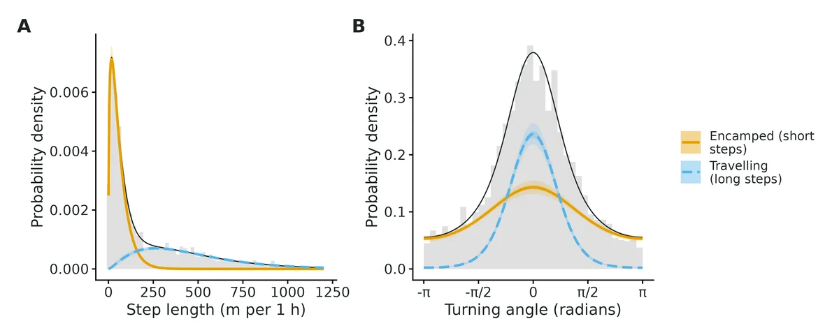
- Encamped (short steps): mean step 60 m per 1 h (95% CI 57-63 m), turning concentration 0.50 (0.43-0.57), i.e. little directional persistence (frequent sharp turns and reversals).
- Travelling (long steps): mean step 454 m per 1 h (95% CI 434-473 m), turning concentration 2.32 (2.17-2.49), i.e. moderate directional persistence.
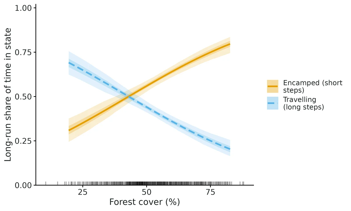
- Activity budget (expected long-run share of time in each state, averaged over the 24-h cycle, at the average value of the habitat covariates): Encamped (short steps) 58% (95% CI 55-61%); Travelling (long steps) 42% (95% CI 39-45%).
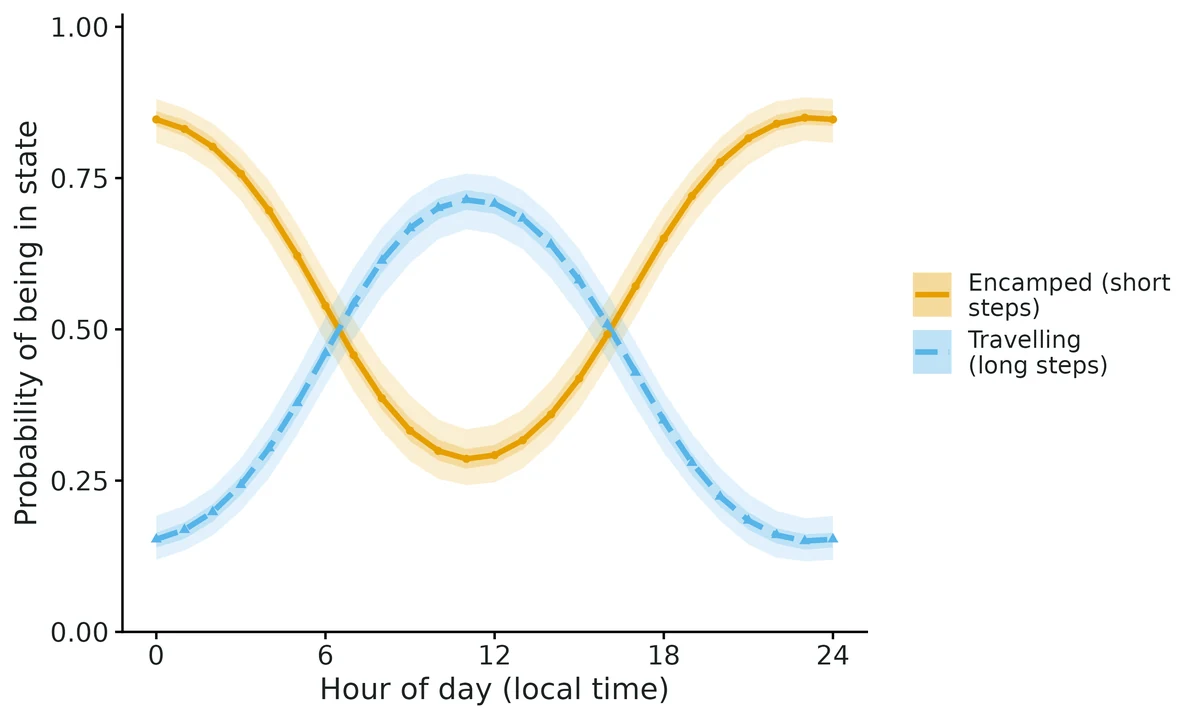
- Time of day: the probability that an animal is in Travelling (long steps) is highest around 11:00 at 71% (95% CI 67-76%) and lowest around 23:00 at 15% (12-19%), with habitat at its mean.
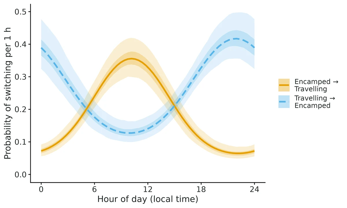
- Each 1-SD increase in forest_cover_pct (14.9 units) multiplies the odds of switching from Encamped to Travelling (versus staying) per time step by 0.67 (95% CI 0.58-0.79); switching back from Travelling to Encamped changes by a factor 1.48 (1.26-1.76) per SD.
- The model-predicted long-run share of time in Encamped (short steps) would be 41% (95% CI 36-47%) if forest_cover_pct were held at 32.5 (10th percentile of the fixes) and 73% (69-77%) if it were held at 72.8 (90th percentile). This is an association with the covariate measured at the animal's location, not proof that forest_cover_pct causes the behaviour.
- States are statistical summaries of movement; labels such as 'resting/foraging' or 'travelling' are interpretations that should be checked against independent observations.
More figures
Figures are the module's default publication figures, reduced for the web. The report also saves them as PDF and full-resolution PNG.
Planted truth at the example's design
Before trusting the example's results, the module was run on many simulated data sets with the same design and known true values. Each row is one quantity: did the method get it back? (What the thresholds are.)
What OPEN means here. The module works (it passes at its default design), but at this example's design not every quantity passed the planted-truth check, so CascadiaTools does not certify those. 15 of the 16 quantities checked passed outright. For tpm 2to1 tod sin, the estimate itself was accurate (within 10% of the truth on average), but the 95% interval was too narrow, containing the truth only 89% of the time. Use those estimates, but read their intervals as somewhat over-confident. The quantities that passed can be used as reported. With your own data, the report would say the same and suggest what would help: more data, a simpler model or a different estimator. More on DONE and OPEN.
Why, for this example:
15/16 estimands pass planted-truth recovery at this design; tpm_2to1_tod_sin coverage 0.890 < bound 0.904 (bias -4.3%, within tolerance). Convergence and GOF pass. Conclusions on states, activity budget and forest association are supported; time-of-day intervals may be slightly narrow (VALIDATION.md Known limit 3).
| This example | 5 elk x 720 hourly GPS fixes, 2 behavioural states, forest cover and time of day on switching |
|---|---|
| Design the module was validated at | 6 animals x 600 hourly fixes, 2 states, time of day and forest cover on switching |
The example has the same total amount of data as the validated default (3,600 hourly fixes), split over 5 animals with longer tracks instead of 6. At the default all 16 estimands passed; the one known weakness is that switching coefficients have slightly narrow intervals (false-positive rate about 7% instead of 5% over 1,596 null tests).
These calls sit close to the pass/fail line. With another 200 simulated data sets they could come out the other way, so read them as “about at the limit” rather than as a clear pass or fail.
- tpm_1to2_tod_sin (✓ PASS): coverage 0.915 against a minimum of 0.904.
- tpm_2to1_tod_sin (✗ FAIL): coverage 0.890 against a minimum of 0.904.
15 of 16 rows pass; 2 are borderline.
Show the full recovery table (16 rows)
| Quantity | True value | Average estimate | Bias | Allowed bias | Coverage (needed) | Result |
|---|---|---|---|---|---|---|
| activity_budget_state1 | 0.592 | 0.593 | +0.2% | ±10.0% | 0.94 (0.904) | ✓ PASS |
| activity_budget_state2 | 0.408 | 0.407 | -0.2% | ±10.0% | 0.94 (0.904) | ✓ PASS |
| step_mean_m_state1 | 60 | 60.1 | +0.2% | ±10.0% | 0.92 (0.904) | ✓ PASS |
| step_mean_m_state2 | 450 | 450.9 | +0.2% | ±10.0% | 0.94 (0.904) | ✓ PASS |
| step_sd_m_state1 | 50 | 50 | -0.0% | ±10.0% | 0.95 (0.904) | ✓ PASS |
| step_sd_m_state2 | 300 | 299.7 | -0.1% | ±10.0% | 0.96 (0.904) | ✓ PASS |
| tpm_1to2_forest | -0.025 | -0.026 | -4.0% | ±10.0% | 0.93 (0.904) | ✓ PASS |
| tpm_1to2_intercept | -1.68 | -1.69 | -0.3% | ±10.0% | 0.96 (0.904) | ✓ PASS |
| tpm_1to2_tod_cos | -0.9 | -0.895 | +0.6% | ±10.0% | 0.95 (0.904) | ✓ PASS |
| tpm_1to2_tod_sin | 0.4 | 0.402 | +0.5% | ±10.0% | 0.92 (0.904) | ✓ PASS ≈ borderline |
| tpm_2to1_forest | 0.025 | 0.0251 | +0.4% | ±10.0% | 0.96 (0.904) | ✓ PASS |
| tpm_2to1_intercept | -1.12 | -1.11 | +0.5% | ±10.0% | 0.95 (0.904) | ✓ PASS |
| tpm_2to1_tod_cos | 0.7 | 0.709 | +1.3% | ±10.0% | 0.95 (0.904) | ✓ PASS |
| tpm_2to1_tod_sin | -0.3 | -0.313 | -4.3% | ±10.0% | 0.89 (0.904) | ✗ FAIL ≈ borderline |
| turn_concentration_state1 | 0.5 | 0.497 | -0.7% | ±10.0% | 0.94 (0.904) | ✓ PASS |
| turn_concentration_state2 | 2.5 | 2.51 | +0.2% | ±10.0% | 0.92 (0.904) | ✓ PASS |
Limits that matter
- Number of states is the analyst's choice; too few states merge behaviours and bias every parameter (VALIDATION.md Known limit 1).
- Transition-coefficient intervals are slightly narrow: null false-positive rate 0.07-0.08 vs 0.05; at this design tpm_2to1_tod_sin covered 0.890 (Known limit 3).
- Missed fixes (5.1%) are treated as missing at random; habitat- or behaviour-dependent fix failure can bias the encamped share and forest association.
- All animals share one set of parameters (no individual random effects, no semi-Markov dwell times) (Known limit 6).
- Habitat effects on switching are associations with conditions at the fix, not causal effects (Known limit 9).
- State labels (encamped/travelling) are interpretations of step length and turning, not observed behaviours.
All known limits from the module's validation record
- Number of states. A model with too few states converges cleanly but merges behaviours and biases everything (section 5). The module does not choose N for you; AIC tends to over-select states in real data (Pohle et al. 2017). Compare 2 vs 3 states with pseudo-residuals and biology.
- Rare transitions in 3-state models can sit on a boundary (4% of replicates); their coefficients and the 3->1 time-of-day effect failed coverage narrowly (0.879). Interpret 3-state models through activity budgets / stationary probabilities.
- Transition-coefficient intervals are slightly narrow: false-positive rate 0.07-0.08 at nominal 0.05 (0.069 pooled over 1596 null tests in four null studies, section 11); coverage of covariate slopes 0.92-0.98; one time-of-day coefficient at 0.889 with 2-h fixes (section 10).
- Short tracks (~450 steps in total): time-of-day coefficients biased up to +17%; forest power ~0.37; 4% of fits have a singular Hessian. Weakly separated states: forest power ~0.43 and borderline coverage for the longer-step state's mean.
- Only gamma step lengths (with an automatic zero-mass when zero steps occur) and von Mises turning angles with mean 0 are built in. The zero-mass branch passed one recovery study (independent simulator, 6% / 1% zero steps; section 10).
- Pooled parameters across animals: no individual random effects; no hidden semi-Markov dwell times.
regularise: crawluses a single best crawl prediction, ignoring location uncertainty (no multiple imputation). On a strongly irregular test set it shortened steps by 10-18% and doubled turning concentrations (section 9); the angle pseudo-residual test flags it. Treat it as a last resort; for irregular data useMIfitHMMoutside the module. Fix interval is estimated as the most common gap between fixes and snapped to a standard schedule; setdata: interval_hif the collar schedule is unusual.- momentuHMM's reported log-likelihood is offset by ~0.1-0.8 units relative to moveHMM because it applies Gamma(1) to the initial distribution (delta is the distribution one step before the first fix; sections 6 and 10). Harmless for estimation, but never mix engines in AIC tables.
- Habitat effects on switching are associations with conditions at the fix, not causal effects.
How this module was validated
- 200 simulated datasets at the default design, fitted by maximum likelihood with momentuHMM (4 starting values); PASSED all 16 estimands (bias at most 2.8%, coverage 0.924-0.990), re-run with the final code at 200/200 converged.
- Harder designs: a 3-state model passed all 36 estimands on re-run; short tracks (3 animals x 150 fixes) and weakly separated states each failed one switching coefficient (bias about +17% or +16%).
- Negative control: fitting 2 states to 3-state data failed 12 of 16 estimands (step means +38% and +131%), showing the gate can fail even when fits look numerically healthy.
- False-positive control with no forest effect passed; pooled over four null studies the interval excluded zero in 0.069 of 1,596 tests (nominal 0.05).
- Cross-check against a hand-written likelihood and moveHMM: all 14 parameters agreed within 0.014 standard errors.
- Power over track length: about 400 hourly fixes per animal (6 animals) needed for 80% power on the forest effect; at 100 fixes slopes were biased up to 19%.
- Two separate verification passes with independent simulators (2-hour fixes with daylight saving; 30-minute fixes with two covariates) passed 15/16 and 18/18; the verifiers fixed the activity-budget definition and a spurious no-standard-error bug; verdict: verified with limits.
Every run uses the acceptance gate described on the validation page. The full record follows, section by section, exactly as kept in the module's VALIDATION.md.
Settings and pass/fail rule used for every run
All runs 2026-10-18/19, R 4.5.3, momentuHMM 1.5.8, moveHMM (cross-check only), on njobvu/chinook via bin/ejob with 16 cores. Reproduce everything with bash dev/movement-hmm/run_validation.sh (configs in modules/movement-hmm/validation/, outputs in results/movement-hmm/validation/<run>/; re-runs after the section-10 activity-budget fix in results/movement-hmm/verify/postfix_<run>/). Recovery uses fast_settings (4 starting values, 1000 parameter draws, no Viterbi/pseudo-residuals). Replicate r uses seed 100000 + r.
Gate (core recovery_gate, unchanged): |bias| <= max(10% of |truth|, 3 MC SE); 95% coverage >= 0.95 - 3 MC SE (floor 0.80); >= 90% of replicates converged. "Converged" = nlm code 1-3 and an invertible Hessian (otherwise no intervals exist; such replicates are excluded from bias and coverage and counted as failures in the convergence criterion). This is a likelihood module, so there is no R-hat; the "R-hat < 1.05" requirement of the build brief is replaced by this rule.
Simulation model (simulate_tracks): correlated random walk with gamma steps and von Mises turns on a smooth 20 x 20 km % forest surface; switching depends on cos/sin of the hour and the forest value at the animal's location; 5% failed fixes and +/-2 min fix-time jitter, so the grid regularisation code is exercised in every replicate. Truth for the transition intercept is expressed at the covariate mean used by fit(); the activity-budget truth is computed from the true parameters with the same function used for the estimate.
Verdict
| design | reps (conv.) | result |
|---|---|---|
| default 2 states, 6 animals x 600 hourly fixes, time of day + forest on switching | 200 (198) | PASS all 16 estimands |
| independent simulator (other author; 2-h fixes, local time with DST, elevation covariate) | 150 (144) | 15/16 PASS; tpm_1to2_tod_sin coverage 0.889 vs bound 0.896 (borderline) |
| independent simulator with zero-length steps (zero-mass branch) | 100 (96) | PASS all 18 incl. zero-step probabilities |
| second independent simulator (30-min fixes, 2 covariates, lon/lat CSV; section 11) | 120 (120) | PASS all 18; null run 200 (200) PASS all 18, null rejection 0.071 |
| default / null / 3-state / short / weak re-run with current code (section 11) | 16/16, 16/16, 36/36, 15/16, 15/16; convergence 99-100% | |
| false-positive control: forest effect = 0 | 200 (199) | PASS all 16; rejection rate of the null 0.080 (1->2) and 0.070 (2->1) |
| 3-state model on 3-state data (6 x 1000 fixes) | 100 (99) | 35/36 PASS; tpm_3to1_tod_sin coverage 0.879 vs bound 0.884 (borderline) |
| harder: short tracks (3 animals x 150 fixes) | 200 (192) | 15/16 PASS; tpm_2to1_tod_cos bias +17.5% (MC SE 4.3%) |
| harder: weakly separated states (100 vs 200 m, kappa 0.8 vs 1.5) | 200 (196) | 15/16 PASS; step_mean_m_state2 coverage 0.903 vs bound 0.903 (borderline) |
| negative control: 2-state model on 3-state data | 100 (98) | FAILS as required: 12/16 estimands fail; step means +38% / +131%, activity budget coverage 0.00-0.03 |
The module is DONE at the default 2-state design (and the 3-state design except one time-of-day coefficient of a rare transition). The harder designs mark its limits (below). No threshold was changed.
1. Default design
Truth: step means 60 / 450 m, SDs 50 / 300 m, turning concentration 0.5 / 2.5; forest slopes -0.025 (1->2) and +0.025 (2->1) per % forest. Median 62 s per replicate (4 starts).
| estimand | truth | mean est. | rel. bias | coverage | CI width |
|---|---|---|---|---|---|
| step_mean_m_state1 | 60 | 60.12 | +0.2% | 0.975 | 5.8 |
| step_mean_m_state2 | 450 | 450.6 | +0.1% | 0.960 | 38.3 |
| step_sd_m_state1 | 50 | 50.04 | +0.1% | 0.975 | 6.4 |
| step_sd_m_state2 | 300 | 299.8 | -0.1% | 0.960 | 33.9 |
| turn_concentration_state1 | 0.5 | 0.498 | -0.5% | 0.944 | 0.146 |
| turn_concentration_state2 | 2.5 | 2.508 | +0.3% | 0.949 | 0.360 |
| tpm_1to2_intercept | -1.685 | -1.688 | -0.2% | 0.990 | 0.340 |
| tpm_1to2_tod_cos | -0.9 | -0.908 | -0.9% | 0.955 | 0.446 |
| tpm_1to2_tod_sin | 0.4 | 0.393 | -1.8% | 0.960 | 0.430 |
| tpm_1to2_forest (per %) | -0.025 | -0.0257 | -2.8% | 0.949 | 0.021 |
| tpm_2to1_intercept | -1.115 | -1.106 | +0.8% | 0.949 | 0.332 |
| tpm_2to1_tod_cos | 0.7 | 0.705 | +0.8% | 0.949 | 0.460 |
| tpm_2to1_tod_sin | -0.3 | -0.301 | -0.3% | 0.949 | 0.422 |
| tpm_2to1_forest (per %) | 0.025 | 0.0250 | -0.1% | 0.939 | 0.022 |
| activity_budget_state1 | 0.592 | 0.594 | +0.3% | 0.924 | 0.063 |
| activity_budget_state2 | 0.408 | 0.407 | -0.4% | 0.924 | 0.063 |
Coverage bound 0.904. Power to exclude zero for the forest slopes: 0.995 (1->2), 0.985 (2->1). 2/200 replicates had a singular Hessian (no intervals). Label switching: states are ordered by mean step length after fitting; no replicate showed swapped states (the step-mean RMSE is 1.4 m and 9.3 m, which would be hundreds of metres under a swap).
2. False-positive rate (forest effect = 0; 200 replicates)
All 16 estimands PASS (coverage 0.915-0.975). The 95% interval of the forest slope excluded 0 in 16/199 (0.080) replicates for 1->2 and 14/199 (0.070) for 2->1; pooled 30/398 = 0.075 (binomial 95% CI 0.05-0.11) against a nominal 0.05. Coverage of these slopes was 0.920 and 0.930: the Wald/delta intervals of transition coefficients are slightly too narrow (empirical SD 0.0056 vs mean reported SE 0.0051-0.0054, about 4-8% too small). Treat a forest effect whose interval only just excludes zero with caution; the report says so in Known limits.
3. Three-state model on three-state data (100 replicates)
Resting / foraging / travelling (step means 30 / 200 / 700 m, kappa 0.3 / 1.0 / 4.0), 6 animals x 1000 fixes, 36 estimands. Median 656 s per replicate (more starts would be slower still: 3-state fits are ~10x the 2-state cost). 35/36 PASS (re-run after the activity-budget fix, section 10; earlier text said 34/35, a miscount). All state-dependent parameters: |rel. bias| <= 0.7%, coverage 0.90-0.99. Activity budgets: bias <= 0.001, coverage 0.919-0.960 (bound 0.884). Forest slopes 1->2 / 2->1: rel. bias -5.7% / -0.5%, coverage 0.94 / 0.96, power 0.92 / 0.90.
Failure: tpm_3to1_tod_sin coverage 0.879 vs bound 0.884 (bias +0.065, truth 0). The 3->1 transition (travelling directly to resting) is rare (truth intercept -3): in 4/99 replicates its intercept went to the boundary (estimates -6.2, -10.1, -102, -695), with huge or no SEs. The mean bias of tpm_3to1_intercept (-1.19) and tpm_3to1_tod_cos (+1.03) is driven entirely by these replicates (median intercept -3.09 vs truth -3.0); they pass the bias rule only because the MC SE is large. Rare transitions in 3-state models are poorly identified; their coefficients must not be interpreted when their SE is large. Interpretation should be via activity budgets and stationary probabilities, which pass.
4. Harder designs (200 replicates each)
Short tracks (3 animals x 150 hourly fixes = ~430 steps; median 19 s/replicate): 15/16 PASS. State parameters fine (|rel. bias| <= 0.9%, coverage 0.92-0.98). Fails tpm_2to1_tod_cos bias +0.122 (+17.5%, MC SE 0.030; tolerance max(0.07, 0.090)): the usual small-sample bias of MLE logit coefficients. 8/200 replicates (4%) had a singular Hessian. Power for the forest slopes falls to 0.375 / 0.365.
Weakly separated states (step means 100 vs 200 m, SDs 80 vs 150, kappa 0.8 vs 1.5; median 75 s/replicate): 15/16 PASS. Fails step_mean_m_state2 coverage 0.903 (bound 0.9031; bias +1.2%): borderline. Activity budget unbiased (+0.04%) but SD 0.069 (vs 0.019 at default) with coverage 0.934. Forest power 0.43. 4/200 singular Hessians.
5. Negative control: 2-state model fitted to 3-state data (100 replicates)
Same 3-state data as section 3, fitted with nstates: 2. Truth for the comparison is the 3-state truth for states 1-2 (the question is whether the gate notices that the model is wrong).
| estimand | truth | mean est. | rel. bias | coverage |
|---|---|---|---|---|
| step_mean_m_state1 | 30 | 41.3 | +38% | 0.00 |
| step_mean_m_state2 | 200 | 461.6 | +131% | 0.00 |
| turn_concentration_state2 | 1.0 | 1.95 | +95% | 0.00 |
| activity_budget_state1 | 0.346 | 0.422 | +22% | 0.03 |
| activity_budget_state2 | 0.373 | 0.578 | +55% | 0.00 |
| tpm_2to1_intercept | -1.456 | -1.904 | -31% | 0.03 |
12/16 estimands FAIL: the 2-state model merges foraging with travelling, so every state's parameters and the activity budget are wrong while all fits "converge" (98/100). The gate can fail. Relevance for users: an HMM with too few states looks perfectly healthy numerically; the pseudo-residual checks and biological judgement (Pohle et al. 2017) are what catch it.
6. Cross-check against independent implementations
dev/movement-hmm/crosscheck.R (log logs/movement-hmm_crosscheck2.log, table dev/movement-hmm/crosscheck_table.csv), default design, seed 4242, ~3,500 steps. The module (momentuHMM, 10 starts) vs (a) a hand-written forward-algorithm likelihood in base R maximised with nlminb (no momentuHMM code), and (b) moveHMM::fitHMM (Michelot et al. 2016).
| parameter | momentuHMM (SE) | hand-written | moveHMM | max diff / SE |
|---|---|---|---|---|
| step mean 1 / 2 (m) | 60.52 (1.35) / 453.01 (9.83) | 60.52 / 453.00 | 60.52 / 452.99 | 0.0017 / 0.0021 |
| step SD 1 / 2 (m) | 49.23 / 301.85 | 49.22 / 301.86 | 49.22 / 301.86 | 0.0016 / 0.0014 |
| kappa 1 / 2 | 0.4416 / 2.5019 | 0.4416 / 2.5018 | 0.4416 / 2.5018 | 0.0003 / 0.0010 |
| 8 transition coefficients | 0.0011-0.0137 |
All 14 parameters agree within 0.014 standard errors; standard errors of momentuHMM and the hand-written Hessian agree within 0.2%. Log-likelihoods: hand-written and moveHMM identical (-24683.0995); momentuHMM reports -24682.9678, 0.13 higher. We checked that momentuHMM's gamma and von Mises densities equal base R's to machine precision (max |log ratio| < 4e-16) and that covariates enter at time t (lagging them by one step changes the likelihood by 11 units). Explained by the independent verification (section 10): momentuHMM starts each animal's forward recursion with delta Gamma(1) P(x_1) (delta is the state distribution one step BEFORE the first fix), whereas moveHMM and the hand-written likelihood use delta P(x_1); a hand-written forward pass with momentuHMM's convention reproduces its log-likelihood to 1e-6. The two are different parameterisations of the nuisance initial distribution. It does not move the estimates, but do not compare momentuHMM log-likelihoods/AIC with those from moveHMM; within the module all comparisons use momentuHMM.
7. Power over track length
6 animals, hourly fixes, default effect (forest slope -0.025 / +0.025 per %; 1 SD of forest is ~15 % so the odds ratio per SD is ~0.69 / 1.45).
| fixes per animal | power 1->2 forest | power 2->1 forest | coverage (1->2 / 2->1) | rel. bias (1->2 / 2->1) |
|---|---|---|---|---|
| 100 | 0.55 | 0.45 | 0.91 / 0.97 | -19% / +13% |
| 200 | 0.76 | 0.67 | 0.93 / 0.91 | -5% / -4% |
| 400 | 0.98 | 0.95 | 0.92 / 0.93 | -9% / -4% |
| 800 | 1.00 | 1.00 | 0.92 / 0.93 | -1% / +7% |
About 400 hourly fixes per animal (6 animals, ~17 days each) are needed for 80% power at this effect size; at 100 fixes the slopes are also biased by up to 19%.
8. Worked example
elk_gps.csv is simulated (5 elk x 720 hourly fixes, lon/lat WGS84 in the Oregon Coast Range, local timestamps, failed fixes absent; generator dev/movement-hmm/make_example.R, truth in example_truth.rds). Fitted with the default settings (10 starts; 10/10 reached the same optimum; pseudo-residual KS p = 0.93 (steps), 0.75 (angles); lag-1 ACF -0.02). 15 of 16 95% intervals contain the truth (e.g. forest 1->2 -0.0265 [-0.0365, -0.0160], truth -0.025; activity budget encamped 0.582 [0.549, 0.611], truth 0.586; re-fitted 2026-10-19 after the section-10 fix, report results/movement-hmm/example/movement-hmm_report.html). The miss is the travelling turning concentration, 2.32 [2.17, 2.49] vs 2.5, consistent with the 95% nominal rate.
9. Irregular fixes
Test set dev/movement-hmm/crawl_test/ (built by dev/movement-hmm/make_crawl_test.R): 3 of the example elk, 30% of fixes deleted and every fix time jittered uniformly +/-25 min around the hourly schedule (an extreme, Argos-like irregularity; GPS jitter is usually seconds to minutes). Same truth as the example. One dataset only, so these are smoke tests, not a recovery study.
Bug found and fixed here. The fix interval was taken as the median gap between fixes; with 30% lost fixes this gave 77 min for a 60-min schedule, so every step was predicted over 1.28 h and the step means were inflated (crawl: 71 / 472 m). The interval is now the most common gap, snapped to a standard schedule within 10% (guess_interval() in hmm_engine.R), and the report states the value used. Checked: 60 min on 5 simulated default datasets, 60 min on the example and on this test set, 4 h on simulated 4-h data with 30% missing. Simulation replicates are unaffected (they pass interval_h explicitly).
| estimand | truth | crawl (1 h) | grid, tolerance 0.45 |
|---|---|---|---|
| step_mean_m_state1 | 60 | 53.8 [50.7, 57.1] | 74.7 [66.1, 84.1] |
| step_mean_m_state2 | 450 | 369.8 [354, 385] | 513.6 [460, 569] |
| turn_concentration_state1 | 0.5 | 1.05 [0.95, 1.16] | 0.46 [0.27, 0.75] |
| turn_concentration_state2 | 2.5 | 3.40 [3.11, 3.73] | 2.15 [1.70, 2.73] |
| tpm_1to2_forest (per %) | -0.025 | -0.0275 [-0.041, -0.014] | -0.047 [-0.074, -0.018] |
| tpm_2to1_forest (per %) | 0.025 | 0.0178 [0.004, 0.033] | 0.013 [-0.009, 0.039] |
| activity_budget_state1 | 0.587 | 0.517 [0.472, 0.561] | 0.612 [0.544, 0.672] |
| angle pseudo-residual KS p | 0.000 | 0.90 |
crawl's own fit is stochastic (simulated-annealing starts): a repeat run gave step means 54.4 / 374.5 m, so crawl-based results can shift slightly between runs.
Neither route is unbiased with this much timing error. The single crawl prediction smooths the path: steps are too short (-10% / -18%) and turning is far too directed (kappa doubled), the activity budget interval misses the truth, and the angle pseudo-residual test rejects (p < 0.001), so the module's own check flags the problem. The grid route drops 229 fixes (off-grid) and leaves 45% of time steps missing; steps are inflated (+24% / +14%, because the real time between "hourly" fixes varies from 10 to 110 min) and the intervals are wide: 5 of 7 contain the truth (both step means are missed). Conclusion: for GPS data with small timing jitter use the default grid; for strongly irregular data neither option here is adequate; use multiple imputation (momentuHMM MIfitHMM) outside this module.
10. Independent verification (2026-10-19)
A second pass by a separate author, using scripts in dev/movement-hmm/verify/ and outputs in results/movement-hmm/verify/. Findings and what changed:
(a) Activity-budget definition fixed. The activity budget was the average of the hour-specific stationary distributions (as in moveHMM's plotStationary). With time of day on the transitions the chain is periodic, and that average is not the long-run share of time. It is now the periodically stationary distribution (Koslik et al. 2025) averaged over the fixes of one day, on the actual fix schedule (interval_h, first-fix phase), in periodic_probs() / activity_budget() in hmm_engine.R; the same function gives the simulation truth, the stationary_tod curve and the habitat curves. dev/movement-hmm/verify/periodic_check.R checks it against a brute-force simulation of the state chain (log logs/movement-hmm_verify_periodic.log): the new definition matches the simulated long-run shares to <= 0.001 in all three test cases (default 0.5648 vs simulated 0.5648; 3-state 0.333/0.377/0.291 vs 0.332/0.378/0.291; strong daily cycle 0.5401 vs 0.5403), whereas the old average was off by up to 0.018 (3-state state 1: 0.351). The default, null, 3-state and negative-control studies were re-run after the fix (results/movement-hmm/verify/postfix_*); sections 1, 2, 3 and 5 report the re-run numbers. Only the activity-budget rows changed (default coverage 0.944 -> 0.924; all other estimands identical to the pre-fix run because the fits are the same). The harder designs (section 4) and the power run (section 7) were not re-run; their activity-budget numbers use the old definition, and their listed failures concern other estimands.
(b) Independent simulator (indep_sim.R, no module code): 2-h fixes, timestamps in local time with daylight saving (America/Denver), an elevation covariate (m) instead of forest, failed fixes both as missing rows and as rows with blank coordinates/covariate, +/-6 min jitter, the fix interval NOT passed (the module must guess it), uniform initial state; 4 animals x 900 fixes; step means 120 / 900 m, kappa 1 / 4; elevation slopes +0.0025 / -0.003 per m.
| run | reps (conv.) | result |
|---|---|---|
| main | 150 (144) | 15/16 PASS. Fail: tpm_1to2_tod_sin coverage 0.889 vs bound 0.896 (bias -0.018 = -2.2%, MC SE 0.014; empirical SD 0.164 vs mean SE 0.140). Elevation slopes: rel. bias -4.7% / -4.4%, coverage 0.958 / 0.979, power 0.81 / 0.99. Activity budget bias +0.0009, coverage 0.944. |
| zero-length steps (6% / 1% zeros) | 100 (96) | PASS all 18; zero-step probabilities 0.0612 (truth 0.06) and 0.0099 (0.01), coverage 0.917 / 0.958. This is the only recovery study of the zero-mass branch. |
| null (elevation effect 0) | 200 (198) | PASS all 16; interval excluded 0 in 0.086 (1->2) and 0.030 (2->1) of replicates, pooled 23/396 = 0.058. |
Convergence (invertible Hessian) was 96% in the main and zero runs, above the 90% rule but lower than with hourly fixes. The time-of-day coefficient failure is the same pattern as Known limit 3 (transition-coefficient SEs ~5-15% too small).
(c) Other checks (checks.R, log logs/movement-hmm_verify_checks.log): the log-likelihood offset vs moveHMM is fully explained by momentuHMM's delta Gamma(1) P(x_1) start (hand-written forward pass reproduces -24682.967752 exactly); the module's 3-state transition-matrix layout matches momentuHMM's own trMatrix_rcpp exactly (max |diff| 0).
(d) Data-entry robustness (messy.R, 11 broken variants of the example CSV): wrong time/id/lat/covariate column names, wrong time format, lon/lat swapped -> read_data stops with a message naming the problem and the fix; misspelled animal id (flagged as a probable typo of elk_F02), text in the covariate, unreadable timestamps (file line numbers given) and duplicated fixes -> check_data reports them; NA coordinates/covariates are accepted as failed fixes.
11. Independent verification, second pass (2026-10-19/20)
A further verifier (scripts dev/movement-hmm/verify/v2_sim.R, v2_run.R, dev/movement-hmm/verify3/, dev/movement-hmm/verify4/; outputs results/movement-hmm/verify3/, verify4/, verify5/; logs logs/movement-hmm_verify{3,4,5}_*). This pass was interrupted once and resumed; all numbers below are from runs made with the current code (module code last changed 2026-10-19 13:59, output.R text-only changes afterwards).
Literature / model check. The model (gamma steps with mean/sd parameterisation, von Mises turns with mean 0, multinomial-logit transitions with staying as reference, covariates of row t driving s_{t-1} -> s_t, working parameters log/log/log/logit) matches Langrock et al. (2012) and the momentuHMM conventions. Rather than relying on documentation, the likelihood was re-implemented by hand (verify4/hess_check.R): it reproduces momentuHMM's log-likelihood to 1.2e-10 on 32 data sets, and the SEs from momentuHMM's nlm Hessian agree with a Richardson-extrapolated numDeriv Hessian of the hand-written likelihood to within 0.1% (median ratio 1.0000). So the slightly narrow transition-coefficient intervals (Known limit 3) are a finite-sample property of Wald intervals, not a numerical Hessian error. The simulator (simulate_tracks) shares only tpm_from_eta/tod_cols with fit-side code; tpm_from_eta's cell order was checked against momentuHMM's trMatrix_rcpp (section 10c), and the independent simulators below share no module code at all.
(a) Bug fixed: spurious "no standard errors" (in hmm_draws(), hmm_engine.R). When the initial-state distribution delta was on a boundary (e.g. every animal starts in the same state), the full Hessian is singular but solve() sometimes "succeeded", returning a numerically rank-deficient inverse; chol() then failed and the replicate was reported as having no intervals (~8% of fits in the second independent design; 2/200 at the default design, 8/200 in short tracks). The module now checks positive definiteness with a relative eigenvalue tolerance and conditions on delta (a nuisance parameter) when it is on a boundary, and also on zero-step probabilities estimated at ~0 (one zero step in the data switches the zero-mass branch on for all states). A note in the report says so. After the fix: default 200/200 converged (was 198), short tracks 200/200 (was 192), weak states 200/200 (was 196).
(b) Second independent simulator (v2_sim.R, no module code; data written as a WGS84 lon/lat CSV in southern-hemisphere UTM 37S and read back through read_data()): 30-min fixes at hh:15/hh:45 local time (Africa/Nairobi), shuffled file order, day-first timestamps, TWO habitat covariates (grass fraction 0-1, distance to water km), every animal starting in state 1, 7% failed fixes, +/-3 min jitter, 1% extra off-schedule fixes that must be dropped, interval not supplied; 5 animals x 1400 fixes; step means 35 / 380 m, kappa 0.3 / 5; activity budget truth by brute-force iteration of the periodic chain.
| run | reps (conv.) | result |
|---|---|---|
| main (effects -1.5/+2.0 per grass unit, +0.12/-0.10 per km) | 120 (120) | PASS all 18; habitat slopes rel. bias +1.1% / +1.2% / -0.6% / +0.3%, coverage 0.925-0.967, power 1.00; activity budget bias -0.0001, coverage 0.958 |
| null (both habitat effects 0) | 200 (200) | PASS all 18; intervals excluded 0 in 0.080 / 0.075 / 0.060 / 0.070 of replicates (pooled 0.071) |
| first verifier's simulator with zero steps (re-run post-fix) | 100 (100) | PASS all 18; zero-step probabilities 0.0611 (truth 0.06) / 0.0098 (0.01), coverage 0.91 / 0.96 |
(c) Builder's studies re-run with the current code (results/movement-hmm/verify3/default, verify4/*, verify5/*):
| design | reps (conv.) | result |
|---|---|---|
| default | 200 (200) | PASS all 16 (coverage 0.925-0.985; forest power 0.995 / 0.985) |
| null forest | 200 (200) | PASS all 16; null rejection 0.080 / 0.070 |
| 3 states | 100 (99) | PASS all 36 (tpm_3to1_tod_sin coverage now 0.889 vs bound 0.884) |
| negative control (2-state on 3-state data) | 100 (100) | FAILS as required, 12/16 estimands (step means +38% / +131%, budget coverage 0.00-0.03) |
| short tracks | 200 (200) | 15/16; tpm_2to1_tod_cos bias +16.8% (unchanged limit) |
| weak states | 200 (200) | 15/16; now tpm_2to1_forest bias +16% fails (step-mean coverage 0.905 passes); forest power 0.42 |
False-positive rate. Pooled over all null studies (builder 400 tests, this pass 800, first verifier 396): 110 / 1596 = 0.069 at nominal 0.05. Slightly liberal, consistently so; the report's Limits paragraph now states this ("about 7% instead of 5%") and advises treating borderline effects as weak evidence.
(d) Usability. The example (results/movement-hmm/example/, re-fitted 2026-10-20) was checked number by number against an independent recomputation (verify4/report_numbers.R): odds ratios per SD 0.67 (0.58-0.79) and 1.48 (1.26-1.76), P(travelling) maximum 71% at 11:00 and minimum 15% at 23:00, long-run encamped share 41% at the 10th and 73% at the 90th forest percentile, activity budget 58% / 42% all reproduce. Wording is associational, not causal; the missed-fix paragraph separates GPS fix success (observation) from behaviour. Report text fixes: the covariate sentence now uses the state names instead of "state 1 / state 2", the forest percentiles are taken at actual fixes (not carried-forward gap values), "random starting values" corrected to "starting values" (one is data-driven), and the liberal false-positive rate is stated. Figure fixes: decoded-track points drawn longest-step state first so encamped clusters are visible; covariate captions use the user's figure label; transition-probability legends now use the state names ("Encamped -> Travelling") instead of "State 1 -> 2". All five required figures of docs/FIGURES.md are present (plus coefficients); plotted curves were checked against fit$estimates (e.g. P(1->2) at 00:00 = plogis(-1.633 - 0.921) = 0.072, as drawn). Messy data (verify/messy2.R, 13 variants) gave actionable messages (section 10d plus ISO-8601 'T'/'Z' timestamps, which now parse, and date-only timestamps, which now stop with a clear message instead of silently dropping the clock time).
Verdict of this pass: VERIFIED_WITH_LIMITS: passes at the default design, at two independent designs and in the 3-state model; the limits are Known limits 1-4 (too few states, rare transitions, slightly liberal intervals for switching coefficients, short tracks / weakly separated states).
Engine, references and full details
Engine: momentuHMM (maximum likelihood via nlm, multiple random starts); moveHMM and a hand-written forward-algorithm likelihood used for cross-checks.
References
- Langrock R, King R, Matthiopoulos J, Thomas L, Fortin D, Morales JM (2012) Flexible and practical modeling of animal telemetry data: hidden Markov models and extensions. Ecology 93(11):2336-2342. doi:10.1890/11-2241.1
- McClintock BT, Michelot T (2018) momentuHMM: R package for generalized hidden Markov models of animal movement. Methods in Ecology and Evolution 9(6):1518-1530. doi:10.1111/2041-210X.12995
- Michelot T, Langrock R, Patterson TA (2016) moveHMM: an R package for the statistical modelling of animal movement data using hidden Markov models. Methods in Ecology and Evolution 7(11):1308-1315. doi:10.1111/2041-210X.12578
- McClintock BT, Langrock R, Gimenez O, Cam E, Borchers DL, Glennie R, Patterson TA (2020) Uncovering ecological state dynamics with hidden Markov models. Ecology Letters 23(12):1878-1903. doi:10.1111/ele.13610
- Pohle J, Langrock R, van Beest FM, Schmidt NM (2017) Selecting the number of states in hidden Markov models: pragmatic solutions illustrated using animal movement. Journal of Agricultural, Biological and Environmental Statistics 22(3):270-293. doi:10.1007/s13253-017-0283-8
- Johnson DS, London JM, Lea MA, Durban JW (2008) Continuous-time correlated random walk model for animal telemetry data. Ecology 89(5):1208-1215. doi:10.1890/07-1032.1
- Koslik J-O, Feldmann CC, Mews S, Michels R, Langrock R (2025) Inference on the state process of periodically inhomogeneous hidden Markov models for animal behavior. Annals of Applied Statistics 19(4):2724-2737. arXiv:2312.14583
- Zucchini W, MacDonald IL, Langrock R (2016) Hidden Markov Models for Time Series: An Introduction Using R, 2nd edn. Chapman & Hall/CRC.
