Spatial, multi-species and integrated occupancy (spOccupancy)
Where does the species (or each species of a community) occur, which habitat covariates are associated with occurrence, and is there residual spatial clustering, after accounting for imperfect detection?
Is this the right analysis?
Use it when
Detection/non-detection surveys repeated at sites with known coordinates, when (a) occupancy is likely spatially clustered beyond what the covariates explain (single species, spPGOcc), (b) several species were recorded at the same sites and community-level responses or species richness are wanted (msPGOcc, sfMsPGOcc), or (c) the same species was surveyed with two or more methods (point counts + ARUs, cameras + sign surveys) that should be analysed together (intPGOcc).
Not for
Single-species non-spatial analyses with likelihood output or dynamic (multi-season) occupancy (use occu-single); species interactions (occu-rota / occu-waddle); counts or abundance (N-mixture); estimating the spatial range itself precisely (weakly identified, see Known limits); presence-only data (sdm-presence-only); false-positive detections.
The data you need
Long detection table (site, survey, detected 0/1 [, species] [, method/source] [, survey covariates]); site table with projected x/y coordinates (m or km) and site covariates; optional prediction grid (x, y, same covariates).
What the example's main data file looks like:
| station | week | start_date | days_active | detected |
|---|---|---|---|---|
| CAM-001 | 1 | 2024-06-12 | 7 | 0 |
| CAM-001 | 2 | 2024-06-19 | 7 | 0 |
| CAM-001 | 3 | 2024-06-26 | 7 | 0 |
| CAM-001 | 4 | 2024-07-03 | 7 | 0 |
| CAM-001 | 5 | 2024-07-10 | 7 | 0 |
Not sure? Use the finder to compare modules.
The worked example
Fisher occupancy, canopy cover and elevation with residual spatial clustering (simulated camera-trap survey, 160 stations)
The question: Is fisher occupancy associated with canopy cover and elevation, allowing for missed detections and for residual spatial clustering, and where in the 30 x 30 km block are fishers likely to occur?
The data are simulated, so the true answer is known and the analysis can be checked against it.
What the researcher typed
I have fisher camera-trap data from 160 stations in the western Cascades, summer 2024, up to 6 weekly occasions per camera (some cameras died early). fisher_detections.csv has one row per station-week (station, week, start date, days the camera worked, detected 1/0). camera_stations.csv has UTM coordinates, canopy cover (%), elevation (m) and ownership. prediction_grid_1km.csv is a 1-km grid with the same covariates. Is fisher occupancy related to canopy cover and elevation? Please account for fishers we missed and for spatial clustering, and make a map of predicted occupancy. I need results and figures for a paper.
Run it yourself
Download the example data below and unzip it.
Open the unzipped folder in Claude Code (see Install).
Paste the prompt above. The agent checks the files, writes a plan, runs planted truth, fits the model and writes the report. You can compare your results with the ones below.
Contains fisher_detections.csv, camera_stations.csv, prediction_grid_1km.csv, the settings file (config.yaml), a description of the data and a step-by-step walkthrough.
Study design details
| model | spPGOcc (spatial single-species occupancy, NNGP 15 neighbours) |
|---|---|
| n sites | 160 |
| max surveys | 6 |
| surveys done | 903 |
| prop missing | 0.059 |
| surveys per site | 6: 138; 5: 4; 4: 6; 3: 7; 2: 5 |
| extent km | 30 |
| site spacing km | 1.0-40.3 (5% quantile 4.2) |
| n detections | 140 |
| n sites detected | 70 |
| naive occupancy | 0.4375 |
| prediction cells | 900 |
| mcmc | 3 chains x 50000 iter, burn-in 20000, thin 20 |
Results from the example data
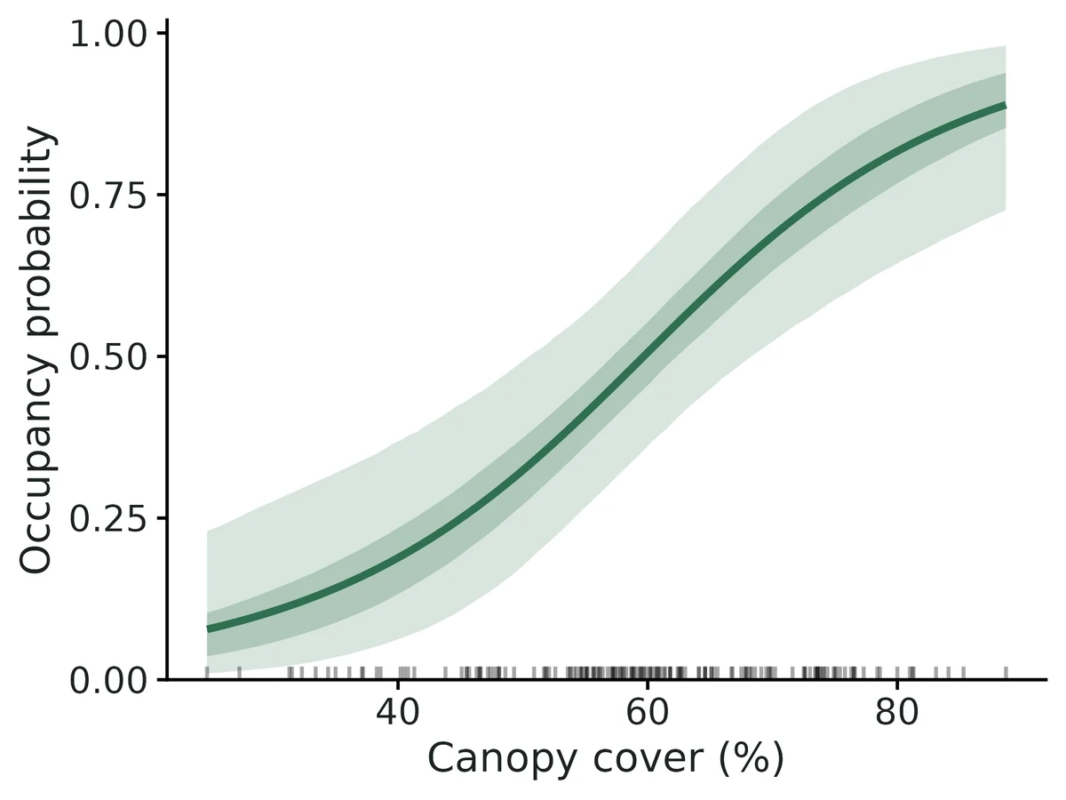
What this means
- Occupancy probability at average covariate values and zero spatial effect is 0.50 (95% CrI 0.36 to 0.65).
- Averaged over the 160 surveyed sites, mean occupancy probability is 0.51 (95% CrI 0.43 to 0.59), and the estimated proportion of surveyed sites that are occupied is 0.51 (95% CrI 0.46 to 0.57), compared with 0.44 of sites where the species was detected at least once (the difference is the correction for missed detections).
- Occupancy and Canopy cover (%): each 1-SD increase (1 SD = 12.9 in original units) multiplies the odds of occupancy by 2.75 (95% CrI 1.65 to 5.26); predicted occupancy goes from 0.28 at 1 SD below the mean to 0.73 at 1 SD above it (other covariates at their means). Per 10-unit increase the odds of occupancy are multiplied by 2.19 (95% CrI 1.48 to 3.64).
- Occupancy and Elevation (m): each 1-SD increase (1 SD = 246 in original units) multiplies the odds of occupancy by 0.58 (95% CrI 0.32 to 0.97); predicted occupancy goes from 0.63 at 1 SD below the mean to 0.37 at 1 SD above it. Per 200-unit increase the odds of occupancy are multiplied by 0.64 (95% CrI 0.40 to 0.98).
- Detection: when the species is present, a single survey detects it with probability 0.30 (95% CrI 0.25 to 0.35) (at average survey conditions).
- Detection and Days camera active in the week: per 1-unit increase the odds of detection are multiplied by 1.48 (95% CrI 1.12 to 2.09). This is a detection effect (how easily the species is found), not a habitat effect.
- The residual spatial variance is 0.95 (95% CrI 0.17 to 3.89) on the logit scale; its prior alone gives a 95% interval of 0.18 to 4.13, so the data add little information: these numbers mostly restate the prior and do not show whether residual clustering is strong or weak.
- Model check: posterior predictive p-values (Freeman-Tukey, by site) are 0.55; no sign of lack of fit.
- All effects are associations from observational data, not causal effects.
More figures
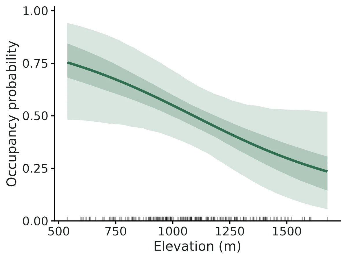
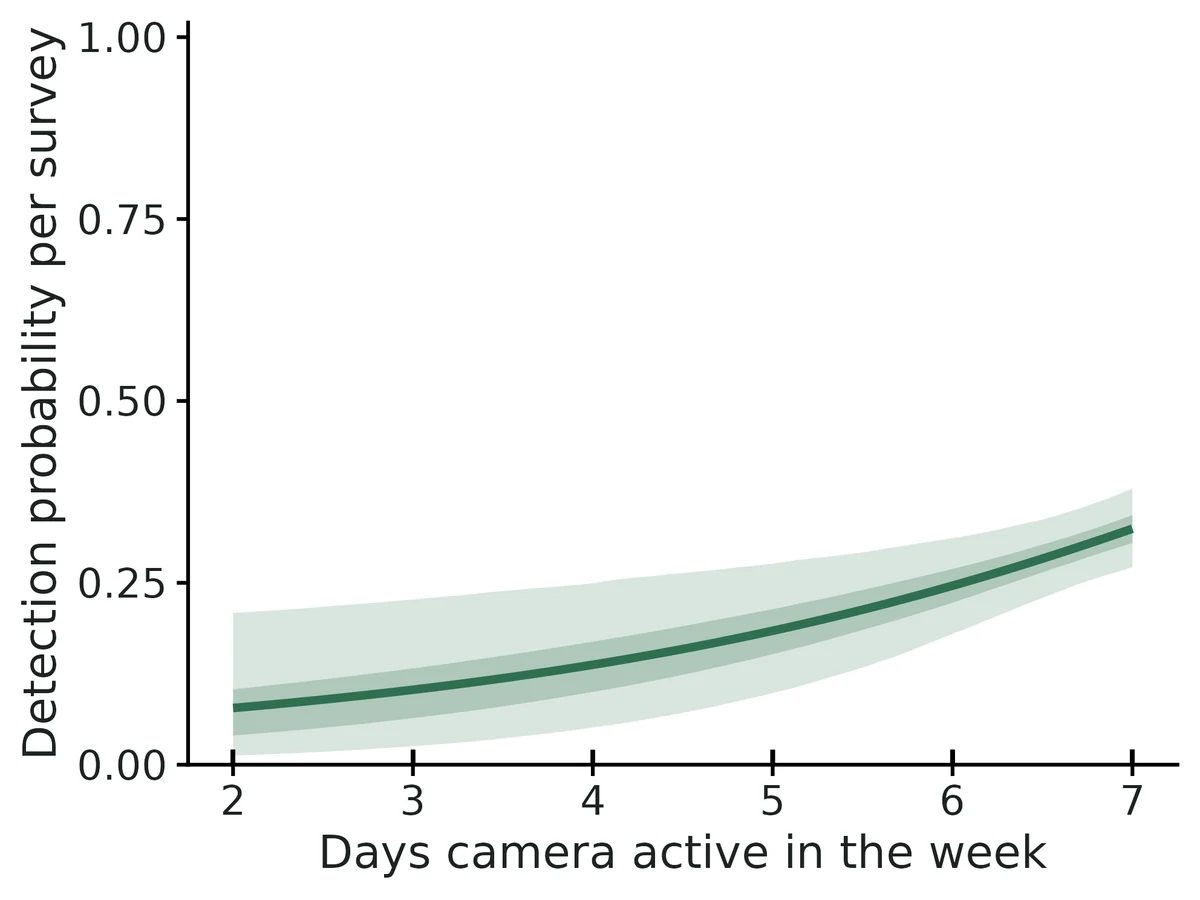
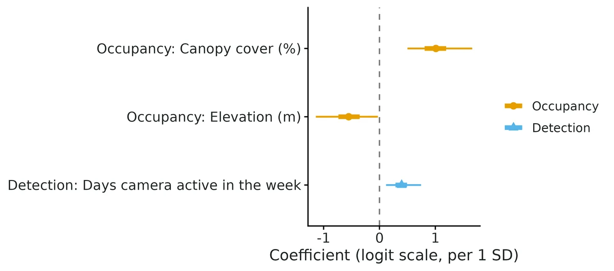
Figures are the module's default publication figures, reduced for the web. The report also saves them as PDF and full-resolution PNG.
Planted truth at the example's design
Before trusting the example's results, the module was run on many simulated data sets with the same design and known true values. Each row is one quantity: did the method get it back? (What the thresholds are.)
DONE for the estimands that answer the question (covariate effects, occupancy, detection, mean occupancy, proportion occupied): all pass planted truth at this design (100/100 converged), the real fit converged and passed the PPC; spatial variance and range fail recovery on bias and are reported descriptively only, not interpreted.
| This example | 160 camera stations, up to 6 weekly surveys, detection about 0.29 |
|---|---|
| Design the module was validated at | 200 sites, 4 surveys, occupancy 0.5, detection 0.4 |
The example has fewer sites (160 vs 200) and lower detection (about 0.29 vs 0.4) than the validated default, though more surveys. VALIDATION.md found that at 100-120 sites with detection 0.25-0.3, occupancy slopes and baseline occupancy were biased 10-28% (coverage stayed 0.95-0.97). At the example's own design the slopes leaned away from zero (+8.2% canopy, -11.5% elevation) and the spatial variance (+48%) and range (+21%) were not recoverable.
These calls sit close to the pass/fail line. With another 100 simulated data sets they could come out the other way, so read them as “about at the limit” rather than as a clear pass or fail.
- psi_beta_canopy_cover_pct (✓ PASS): bias +8.2% against an allowance of ±10.0% (set by the 10% rule), so it used 82% of the allowance.
7 of 9 rows pass; 1 is borderline.
| Quantity | True value | Average estimate | Bias | Allowed bias | Coverage (needed) | Result |
|---|---|---|---|---|---|---|
| occupancy_prob | 0.426 | 0.448 | +5.1% | ±10.0% | 0.93 (0.885) | ✓ PASS |
| psi_beta_canopy_cover_pct | 0.9 | 0.974 | +8.2% | ±10.0% | 0.99 (0.885) | ✓ PASS ≈ borderline |
| psi_beta_elevation_m | -0.4 | -0.446 | -11.4% | ±21.5%† | 0.95 (0.885) | ✓ PASS |
| detection_prob | 0.285 | 0.281 | -1.3% | ±10.0% | 0.96 (0.885) | ✓ PASS |
| p_beta_days_active | 0.38 | 0.38 | +0.1% | ±10.4%† | 0.9 (0.885) | ✓ PASS |
| mean_occupancy | 0.445 | 0.461 | +3.5% | ±10.0% | 0.95 (0.885) | ✓ PASS |
| prop_sites_occupied | 0.452 | 0.461 | +2.0% | ±10.0% | 0.97 (0.885) | ✓ PASS |
| spatial_variance | 1 | 1.48 | +48.1% | ±28.5%† | 1 (0.885) | ✗ FAIL |
| effective_range_km | 8 | 9.7 | +21.3% | ±10.0% | 1 (0.885) | ✗ FAIL |
Limits that matter
- Spatial variance and effective range are not recoverable at this design (+48% and +21% bias in planted truth) and their posteriors restate the priors; read the spatial maps as residual smoothing, not a measured clustering scale.
- Occupancy slopes lean away from zero at modest sample sizes (+8% canopy, +11.5% elevation in planted truth; 10-28% at 100-120 sites in VALIDATION.md; ~10% inflation if no real clustering). Trust direction; report the non-spatial PGOcc fit alongside (canopy 0.87 vs 1.01 per SD).
- Low power for the elevation effect: an effect of -0.40 per SD was detected in only 33% of replicates; the real-data interval only just excludes zero.
- Spatial confounding: smooth covariates such as elevation (15-km range) can have part of their effect absorbed by the spatial term (VALIDATION.md: -20% for a 90%-spatial covariate).
- Recovery simulator differs from the example generator: independent covariates, missing weeks at random rather than camera failures, standard-normal days_active.
- Closure over the season, no false positives and no unmodelled detection heterogeneity are assumed; stations 1 km apart may share individuals, so occupancy is better read as use.
- Core gate caveat: the '>= 90% converged' clause cannot fail for non-convergence; convergence (100/100) was counted by hand.
How this module was validated
- 100 simulated data sets per design with spOccupancy (3 chains x 15000 iterations, 5000 burn-in); at the default design all covariate, occupancy and detection quantities passed, while the spatial range is only descriptive.
- Harder designs: 100 sites x 3 surveys with detection 0.25 failed on occupancy (+13.3%); community models passed on means but community SDs were biased +15-30%; one spatial factor community model converged in only 76 of 100 runs.
- Negative control: fitting a non-spatial model to strongly spatial data biased the forest slope -27.5% (coverage 0.74) and failed the gate; false-positive rates were 0.05-0.07.
- Cross-checks: the simulator matched spOccupancy::simOcc; the non-spatial engine matched unmarked (correlation at least 0.999); a community model matched a hand-written Nimble model.
- Power for a forest effect of 0.8: 0.34, 0.74, 0.90 and 1.00 at 50, 100, 200 and 400 sites.
- A separate verifier with its own simulator found a 120-site failure (slopes -24% and +28%) that disappeared at 480 sites, showed the spatial model inflates slopes on non-spatial data, reproduced the builder's runs exactly, and fixed several silent data problems.
Every run uses the acceptance gate described on the validation page. The full record follows, section by section, exactly as kept in the module's VALIDATION.md.
Settings and pass/fail rule used for every run
Status: VERIFIED WITH LIMITS for spPGOcc (default design), msPGOcc community means and intPGOcc. Not gate-passing: sfMsPGOcc at fast settings (convergence), community SDs (bias), spPGOcc at small or low-detection designs (bias), and the spatial range. spIntPGOcc is not validated.
All recovery runs use fast_settings (3 chains x 15000 iterations, burn-in 5000, thin 10, 10 neighbours, converge_on = "core"). They are gated with the unchanged core/R/recovery.R thresholds:
| bias | <= max(10% of truth, 3 MC SE); coverage >= 0.95 - 3 MC SE (0.885 at nsim 100); >= 90% of reps converged. |
|---|
Gate caveat (core bug, not fixed here): summarise_recovery() sets n_ok to the number of converged reps, so n_converged / (n_ok + n_failed) is always 1 unless a rep errored. The ">= 90% converged" clause therefore never fails for non-convergence. The convergence fractions below were counted by hand from the reps files.
1. Builder's recovery runs
Commands: bash dev/occu-spatial/run_recover.sh <cfg> (config in dev/occu-spatial/<cfg>.yaml).
single_default: spPGOcc, 200 sites x 4 surveys, psi 0.5, p 0.4, sigma^2 1.5, range 6 km
100/100 converged, median 118 s/rep.
| param | truth | mean est | rel. bias | coverage | gate |
|---|---|---|---|---|---|
| occupancy_prob | 0.5 | 0.509 | +1.7% | 0.96 | PASS |
| psi_beta_forest | 0.8 | 0.819 | +2.4% | 0.98 | PASS |
| detection_prob | 0.4 | 0.406 | +1.5% | 0.97 | PASS |
| p_beta_effort | 0.5 | 0.517 | +3.3% | 0.96 | PASS |
| mean_occupancy | 0.5 | 0.503 | +0.9% | 0.94 | PASS |
| prop_sites_occupied | 0.504 | 0.503 | -0.1% | 0.94 | PASS |
| spatial_variance | 1.5 | 1.67 | +11.0% | 0.97 | PASS (descriptive only) |
| effective_range_km | 6 | 7.0 | +16.7% | 1.00 | FAIL bias (weakly identified; descriptive only) |
Power for psi_beta_forest is 0.96.
single_hard: spPGOcc, 100 sites x 3 surveys, p 0.25
100/100 converged. occupancy_prob +13.3% (FAIL bias), mean_occupancy +11.0% (FAIL), prop_sites_occupied +12.1% (FAIL), psi_beta_forest +9.7% (PASS, power 0.40), p_beta_effort +6.1% (PASS), detection_prob -5.2% (PASS). Coverage is 0.95-0.98 for every estimand. The range (+10.8%) and variance (-17.6%) fail on bias.
strong_spatial: spPGOcc, sigma^2 3, range 10 km
97/100 converged. Covariates, occupancy and detection all PASS (psi_beta_forest -2.3%, coverage 0.97).
negctrl_nonspatial: PGOcc fitted to the strong-spatial data (negative control)
psi_beta_forest -27.5%, coverage 0.74 (FAIL); occupancy_prob coverage 0.69 (FAIL). The gate can fail when spatial autocorrelation is ignored.
fpr_zero: spPGOcc with both effects = 0
psi_beta_forest rejection rate 0.07 and p_beta_effort 0.05 (100 reps).
multi_ms: msPGOcc, 15 species, 150 sites
100/100 converged. Community means and mean_site_richness PASS (comm_psi_beta_forest +4.9%, richness +0.5%). comm_sd_p_beta_effort is +16.7% (FAIL bias); comm_sd_detection_logit is +9.5% (PASS).
multi_sf: sfMsPGOcc, 15 species, 150 sites, 1 factor (range 6 km)
Only 76/100 converged (R-hat < 1.05 on community-level estimands). That is below the 90% clause, so the whole design FAILS. The core bug above hid this. Among the converged reps:
- PASS: community means, comm_sd_occupancy_logit, comm_sd_psi_beta_forest and richness;
- FAIL bias: comm_sd_detection_logit +11.3%, comm_sd_p_beta_effort +19.5%, effective_range_km_f1 +24.3%.
integrated: intPGOcc, 150 point counts x 3 + 100 ARU x 5 (50 shared)
100/100 converged. All 8 estimands PASS (psi_beta_forest +6.7%, coverage 0.96).
power over n_sites (50/100/200/400; nsim 50)
Power for psi_beta_forest is 0.34, 0.74, 0.90 and 1.00. At 50 sites p_beta_effort is biased +15.5%.
Cross-checks
Simulator vs spOccupancy::simOcc (400 datasets each, identical coordinates):
- naive occupancy 0.4408 vs 0.4416 (KS p 0.98);
- detection frequency 0.4628 vs 0.4636 (KS p 0.91);
- Moran's I 0.0523 vs 0.0525 (KS p 0.64);
- the covariance function is identical to
mkSpCov(0.2030029 both).
- intPGOcc vs hand-coded marginal ML (48 datasets): mean |difference| 0.0008-0.004 for probabilities and detection slopes, 0.020 for psi_beta_forest; correlation 1.00.
- msPGOcc vs a hand-written Nimble community model (same priors, 3 datasets): mean |difference| is <= 0.008 for every community estimand and 0.006 for richness.
- The builder's chinook jobs for "spPGOcc vs PGOcc vs unmarked on non-spatial data" and for "spPGOcc fitted to simOcc data" hit the SLURM time limit with no output. The non-spatial engine comparison was rerun by the verifier on njobvu (section 2).
- Nimble exact-GP vs spPGOcc: still running on chinook at the time of verification (no result).
2. Independent verification (2026-10-19, separate verifier agent)
What was checked
Literature and package source. I checked spOccupancy 0.8.2 (installed source):
- coefficient priors N(0, var 2.72) and sigma^2 ~ IG(2, 1) match the module;
- phi ~ U(3/max d, 3/min d) is the package default, while the module uses the 5% distance quantile for the lower range bound (deliberate and documented);
- the exponential covariance is sigma^2 exp(-phi d), so effective range = 3/phi (correlation 0.05);
- sfMsPGOcc fixes factor variances at 1 and loadings lower-triangular with unit diagonal, and sim.R matches;
- msPGOcc gives species coefficients N(mu, tau^2) with tau^2 ~ IG(0.1, 0.1), and the module reports sqrt(tau^2).
- Shared code. simulate() and fit() share only
d_or()and the term-naming convention. My independent simulator shares nothing.
Independent planted truth
dev/occu-spatial/verify/vsim.R is my own generator: eigen-decomposition GP draws, jittered-grid sites in UTM metres, ragged 3-6 visits, raw-unit covariates. It writes researcher-style CSVs and reads them back through the module's read_data() → check_data() → fit(), so io, standardisation and estimand naming are also tested. Designs and parameters differ from the builder's. Seeds are 7000 + rep. Results are in results/occu-spatial/verify/<scenario>/summary.csv.
| scenario | design | nsim | converged | result |
|---|---|---|---|---|
| sp | spPGOcc, 120 sites, p 0.3, psi 0.35, sigma^2 1, range 4 km, 2 covariates (elev partly spatial) | 150 | 150 | FAIL: psi_beta_elev -0.866 vs -0.70 (-24%), psi_beta_shrub 0.513 vs 0.40 (+28%), occupancy_prob +10.5%; p_beta_temp coverage 0.88 (bound 0.897). Coverage of both slopes 0.95-0.97. detection_prob, mean_occupancy, prop_occupied PASS |
| spbig | same generator, 480 sites | 100 | 95 | all gated estimands PASS: psi_beta_elev -2.8%, psi_beta_shrub +3.4%, occupancy_prob +3.8%, detection_prob -2.6%, p_beta_temp -2.2% (coverage 0.95), mean_occupancy +2.6%; coverage 0.93-0.98. spatial_variance -7% (PASS); effective_range_km +85% (FAIL, descriptive only) |
| fpr | sp with shrub effect 0 | 200 | 200 | false-positive rate for shrub 0.07 (14/200); psi_beta_elev -14.7% (FAIL bias) |
| neg | PGOcc on strongly spatial data (sigma^2 3, range 10 km) | 100 | 100 | negative control fails, as it should: psi_beta_elev coverage 0.86 (bound 0.885), psi_beta_shrub -20%, occupancy_prob coverage 0.63 |
| negsp | spPGOcc on the same data | 100 | 100 | shrub -0.9%, coverage 0.98 (PASS); elev (90% spatially smooth) -20%, coverage 0.90 (spatial confounding) |
| ms | msPGOcc, 10 species, 100 sites, ragged visits | 100 | 100 | community means and richness PASS (comm_psi_beta_conifer -0.4%); comm_sd_p_beta_effort_h +30%, comm_sd_psi_beta_conifer +18% (FAIL bias, coverage 0.95-0.96) |
| sf | sfMsPGOcc, same with 1 factor | 100 | 97 | community means and richness PASS; comm_sd_occupancy_logit +13%, comm_sd_p_beta +27%, comm_sd_psi_beta +16% (FAIL bias) |
| int | intPGOcc, transects 100 x 2 + cameras 100 x 6 (40 shared), lognormal covariate | 100 | 100 | all 8 PASS (psi_beta_wet +10.8% within 3 MC SE; coverage 0.93-0.97) |
Re-running the builder's commands. recover_integrated reproduced every number exactly (results/occu-spatial/verify/rerun_integrated). recover_single_default rerun with the patched module: identical table (100/100 converged; every mean, coverage and gate outcome matches section 1; results/occu-spatial/verify/rerun_single_default). The fit on example/config.yaml with the patched module also reproduced the builder's estimates exactly (results/occu-spatial/verify/example_fit).
Interpretation of the small-design failure. Same generator, parameters and seeds, but with 4x the sites (480 vs 120):
- psi_beta_elev bias went from -24% to -2.8%;
- psi_beta_shrub went from +28% to +3.4%;
- occupancy_prob went from +10.5% to +3.8%.
So the 120-site failure is small-sample behaviour of the posterior mean (logit slopes pulled away from zero with about 40 occupied sites, p = 0.3 and a spatial random effect), not a module or io bug. The builder's single_hard design (100 sites, p 0.25) shows the same pattern.
Coverage of the slopes stayed at 0.95-0.97 throughout, so the intervals remain honest; only the point estimates lean high. This is recorded as a design limit in README Pitfalls and in the report's "Validated limits" sentence. Users must run recover at their own design.
Engine cross-check on non-spatial data (spec item; builder's job had timed out)
dev/occu-spatial/verify/xc_nonspatial_v.R uses 64 datasets from the default design with sigma^2 = 0. It fits spPGOcc, PGOcc and unmarked::occu to each dataset (results/occu-spatial/verify/xc_nonspatial_engines.csv; log logs/occu-spatial_verify_xc_nonspatial.log).
PGOcc vs unmarked (independent likelihood engine):
- per-dataset correlation >= 0.999 for all four parameters;
- mean |difference|: 0.002 detection_prob, 0.006 occupancy_prob, 0.002 p_beta_effort, 0.026 psi_beta_forest (the posterior mean is slightly larger than the MLE, as expected).
spPGOcc vs PGOcc on the same non-spatial data:
- detection agrees (mean |difference| 0.002-0.003);
- psi_beta_forest is inflated: relative bias +20.8% for spPGOcc vs +8.2% for PGOcc and +5.0% for unmarked; mean |sp - ns| = 0.10; coverage 0.92 vs 0.94.
The IG(2,1) prior keeps sigma^2 away from 0 (median posterior mean 0.66), so the slopes become conditional on a spurious spatial effect. Limit: when the spatial variance posterior merely restates its prior, also fit PGOcc and report both. The report now says this in that case.
Usability (messy copies of the fisher example; dev/occu-spatial/verify/messy.R)
Before the fixes, these problems were handled silently or with unclear messages:
- NA detection values were silently treated as surveys not done;
- duplicated site x survey rows were silently accepted;
- lat/long coordinates were silently accepted (every distance would be ~0 km);
- a misspelled covariate column gave
object 'elevation_m' not found.
All of these now give actionable messages. Missing site or survey covariates, a misspelled site id, non-0/1 values and duplicate coordinates were already caught. The site-id error now suggests the closest match ("'CAM-14' (did you mean 'CAM-014'?)").
Report check (fisher example): every number in the interpretation was recomputed from the estimates table. Examples:
- OR per SD exp(1.010) = 2.75;
- elevation per 200 m exp(-0.551 x 200/246) = 0.64;
- detection per day exp(0.397/1.01) = 1.48;
- the IG(2,1) prior 95% interval is 0.18-4.13.
The report uses association language, keeps detection and habitat effects apart, and gives effects on the probability scale. The conditional-effects curves (occupancy vs canopy; detection vs days active) were inspected: they pass through the reported values at the covariate means and include rug and 50/95% bands.
Changes made by the verifier
R/io.R:- missing-column errors list the file's actual columns and the config key to change;
- formula terms are checked against the file;
- empty detections are dropped with a note;
- duplicate site x survey rows and duplicate site ids are flagged;
- degree-like coordinates are flagged;
- a misspelled site id gets a closest-match suggestion;
- missing survey covariates report a count and example sites.
R/fit.R: data notes are passed into the diagnostics. Withconverge_on = "all", a note is added when R-hat >= 1.01 or bulk ESS < 400 (the real-data standard).R/report.R:- the per-unit odds ratio now uses exp(posterior-mean slope), consistent with the per-SD odds ratio (previously the mean of exp(), e.g. 2.26 vs 2.19);
- the spatial paragraph now compares the spatial-variance interval with its prior interval and fixes the awkward "8.8 (95% CrI ...) km" wording;
- trace panels have readable labels;
- the "Validated limits" sentence now states the measured limits instead of claiming unbiased recovery at all designs.
- Estimation code is unchanged. Originals are kept in
dev/occu-spatial/verify/*.R.orig. R/report.R(later): when the spatial-variance interval matches its prior, the report now recommends also fitting PGOcc (see the engine cross-check above).- Note: these edits were made while the builder's
xc_nimble.R spatialjob (chinook, started 23:07) was still running. That R process had already loaded the module and only usesfit(), which is unchanged, so its results are unaffected.
Verifier verdict: VERIFIED WITH LIMITS
Pass (gated estimands: covariate effects, occupancy, detection, mean occupancy):
- spPGOcc at the default design (reproduced exactly) and at 480 sites on independent data;
- msPGOcc community means and richness (builder's design and independent design);
- intPGOcc (builder's design reproduced exactly; independent design passes).
Controls:
- the negative control (PGOcc on spatial data) fails the gate;
- false-positive rates are 0.07 (independent, 200 reps), 0.07 and 0.05 (builder).
Limits (gate fails, documented):
- spPGOcc at about 100-120 sites with p 0.25-0.3: slope and baseline bias 10-28%, coverage OK;
- spatial range is never gated;
- community SDs +15-30%;
- sfMsPGOcc reached only 76% convergence at fast settings (builder's design); the independent design reached 97%;
- spPGOcc on non-spatial data inflates slopes about 10% relative to PGOcc;
- spIntPGOcc is not validated.
- Open item: Nimble exact-GP vs spPGOcc result still pending (chinook job).
Engine, references and full details
Engine: spOccupancy 0.8.2 (Polya-Gamma Gibbs samplers; NNGP spatial random effects).
References
- Doser JW, Finley AO, Kery M, Zipkin EF (2022) spOccupancy: An R package for single-species, multi-species, and integrated spatial occupancy models. Methods in Ecology and Evolution 13:1670-1678. doi:10.1111/2041-210X.13897
- Doser JW, Finley AO, Banerjee S (2023) Joint species distribution models with imperfect detection for high-dimensional spatial data. Ecology 104(9):e4137.
- Doser JW, Leuenberger W, Sillett TS, Hallworth MT, Zipkin EF (2022) Integrated community occupancy models: a framework to assess occurrence and biodiversity dynamics using multiple data sources. Methods in Ecology and Evolution 13. doi:10.1111/2041-210X.13811
- Datta A, Banerjee S, Finley AO, Gelfand AE (2016) Hierarchical nearest-neighbor Gaussian process models for large geostatistical datasets. JASA 111:800-812.
- Polson NG, Scott JG, Windle J (2013) Bayesian inference for logistic models using Polya-Gamma latent variables. JASA 108:1339-1349.
- Dorazio RM, Royle JA (2005) Estimating size and composition of biological communities by modeling the occurrence of species. JASA 100:389-398.
- MacKenzie DI et al. (2002) Estimating site occupancy rates when detection probabilities are less than one. Ecology 83:2248-2255.
- Banerjee S, Carlin BP, Gelfand AE (2014) Hierarchical Modeling and Analysis for Spatial Data, 2nd ed. CRC Press.
- spOccupancy vignettes (model fitting; factor models), https://doserlab.com/files/spoccupancy-web/
