Two-species conditional occupancy (dominant/subordinate; Richmond et al. 2010, Waddle et al. 2010)
"Is the subordinate species (B) found at fewer sites where the dominant species (A) occurs than where it is absent, and is that pattern stronger in some habitats?", "Is B harder to detect on surveys when A is detected?", after allowing for both species being missed on some surveys.
Is this the right analysis?
Use it when
Repeated detection/non-detection surveys of TWO species at the same sites, where one species can reasonably be treated as dominant (predator, invasive competitor, larger species) and the question is whether the other (subordinate) species occupies sites less (or more) often where the dominant is present, and whether detection of one depends on the other; covariates on every occupancy and detection probability.
Not for
Three or more species, or no defensible dominant/subordinate ordering (use occu-rota, which is symmetric); counts or abundance of the dominant (abund-interactions); single species (occu-single); multi-season colonisation/extinction dynamics.
The data you need
Detection history of both species (site x survey 0/1, both recorded on every survey), site covariates, optional survey covariates.
What the example's main data file looks like:
| site_id | visit | date | observer | air_temp_c | pipes_checked | cuban_treefrog | green_treefrog |
|---|---|---|---|---|---|---|---|
| WCA-001 | 1 | 2023-06-05 | JHW | 22.9 | 10 | 1 | 0 |
| WCA-001 | 2 | 2023-06-29 | MS | 29.6 | 10 | 1 | 0 |
| WCA-001 | 3 | 2023-07-20 | JHW | 21.3 | 10 | 0 | 1 |
| WCA-001 | 4 | 2023-08-09 | MS | 23.7 | 10 | 0 | 0 |
| WCA-001 | 5 | 2023-08-29 | KR | 26.1 | 10 | 0 | 1 |
Not sure? Use the finder to compare modules.
The worked example
Do invasive Cuban treefrogs push out native green treefrogs? Two-species conditional occupancy from PVC-pipe surveys (simulated data)
A crew placed a cluster of 10 PVC pipes at each of 180 sites spread over wetlands and tree islands west of Miami (latitude 25.50-26.00 N, longitude 80.35-80.94 W). Each site was visited 5 times, about every 3 weeks, from 5 June to 31 August 2023. On each visit an observer checked all 10 pipes and recorded whether each species was found in any pipe (1) or not (0), and the air temperature. Some visits did not happen (flooded access, staff shortage): 60 of the 900 planned visits are missing.
The question: Is green treefrog occupancy lower at sites where Cuban treefrogs occur, and is green treefrog detection lower on visits when Cuban treefrogs are found in the pipes, after allowing for both species being missed?
The data are simulated, so the true answer is known and the analysis can be checked against it.
What the researcher typed
I have pipe-survey data for Cuban treefrogs and green treefrogs at 180 sites, 5 visits each, in pipe_surveys.csv, and site information (distance to road, canopy cover) in sites.csv. I want to know whether green treefrogs occupy fewer sites where Cuban treefrogs are present, and whether green treefrogs are harder to detect on visits when Cuban treefrogs are found. Cuban treefrog detection probably depends on air temperature. Please run the analysis and give me a report with figures I can use in a paper.
Run it yourself
Download the example data below and unzip it.
Open the unzipped folder in Claude Code (see Install).
Paste the prompt above. The agent checks the files, writes a plan, runs planted truth, fits the model and writes the report. You can compare your results with the ones below.
Contains pipe_surveys.csv, sites.csv, the settings file (config.yaml), a description of the data and a step-by-step walkthrough.
Study design details
| n sites | 180 |
|---|---|
| n visits per site | 5 |
| visits done | 840 |
| visits missed | 60 |
| prop missing | 0.067 |
| pipes per site | 10 |
| site covariates | log(dist_road_m) on psiA, canopy_pct on psiBA and psiBa |
| survey covariates | air_temp_c on pA and pB |
| sites cuban detected | 90 |
| sites green detected | 81 |
| sites both detected | 23 |
| data simulated | True |
| generator | dev/occu-waddle/make_example.R, set.seed(2010) |
Results from the example data
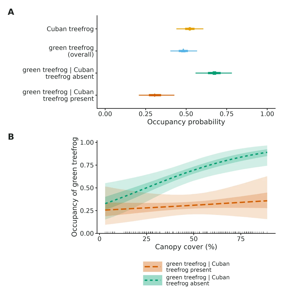
What this means
- Where Cuban treefrog is present, green treefrog occupies 0.31 (95% CrI 0.21 to 0.43) of sites; where Cuban treefrog is absent, 0.67 (95% CrI 0.56 to 0.78).
- The odds of green treefrog occupying a site are 0.21 (95% CrI 0.10 to 0.44) times as high where Cuban treefrog is present.
- The species interaction factor is 0.64 (95% CrI 0.46 to 0.81): at average conditions the two species co-occur less often than expected if they were distributed independently (a segregation pattern).
- Occupancy of Cuban treefrog: the odds are multiplied by 0.40 (95% CrI 0.26 to 0.57) per 1 SD of log(dist_road_m); it decreases from 0.96 at 29 m to 0.09 at 5410 m.
- Occupancy of green treefrog where Cuban treefrog is absent: the odds are multiplied by 2.13 (95% CrI 1.35 to 3.63) per 1 SD of canopy cover (from 0.33 at 3% to 0.89 at 89%); where Cuban treefrog is present there is no clear change (1.14, 95% CrI 0.67 to 1.98).
- Where both occur, green treefrog is detected on 0.23 (95% CrI 0.13 to 0.36) of surveys that detected Cuban treefrog and on 0.50 (95% CrI 0.36 to 0.64) of surveys that missed it; log-odds ratio -1.18 (95% CrI -2.01 to -0.40). This is a detection effect, not an occupancy effect.
- A difference between psiBA and psiBa, or an SIF away from 1, is a co-occurrence pattern, consistent with competition or predation but equally with both species responding to habitat features not in the model; it does not by itself show that Cuban treefrog excludes green treefrog.
More figures
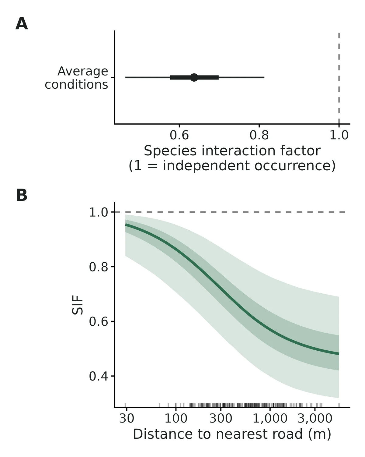
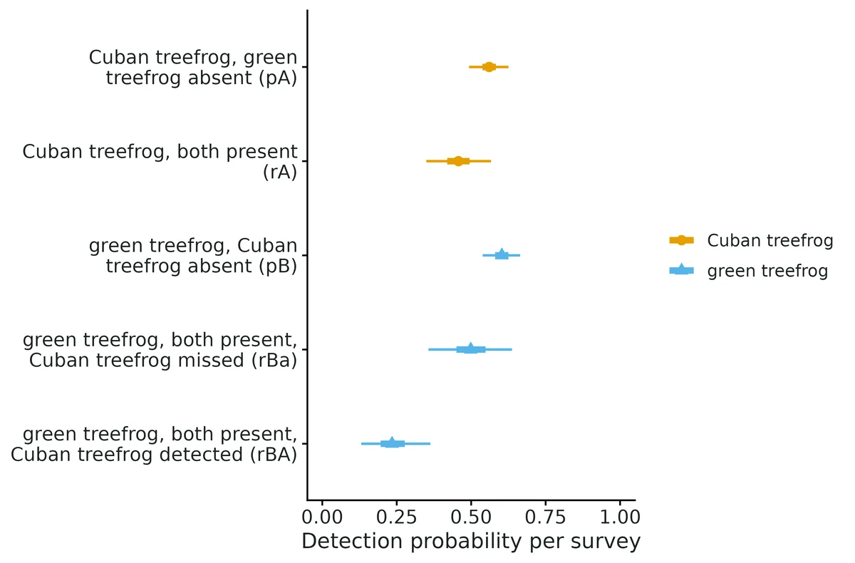
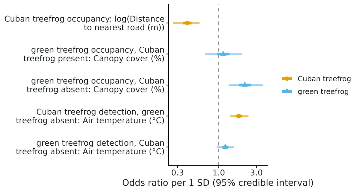
Figures are the module's default publication figures, reduced for the web. The report also saves them as PDF and full-resolution PNG.
Planted truth at the example's design
Before trusting the example's results, the module was run on many simulated data sets with the same design and known true values. Each row is one quantity: did the method get it back? (What the thresholds are.)
Every quantity checked passed planted truth at this design.
| This example | 180 sites, 5 visits each, Cuban and green treefrogs |
|---|---|
| Design the module was validated at | 200 sites, 4 surveys each |
The example is close to the validated default: slightly fewer sites (180 vs 200) but one more visit per site. At this design the interaction quantities were within +-2.5%; VALIDATION.md shows they are biased toward no interaction only at about 60 sites (+12% to +21%). Canopy effects on green treefrog occupancy have low power here (0.39 and 0.53), and the detection interaction has power 0.61.
18 of 18 rows pass.
Show the full recovery table (18 rows)
| Quantity | True value | Average estimate | Bias | Allowed bias | Coverage (needed) | Result |
|---|---|---|---|---|---|---|
| det_dominant_alone | 0.55 | 0.549 | -0.2% | ±10.0% | 0.96 (0.904) | ✓ PASS |
| det_dominant_alone_beta_effort | 0.378 | 0.394 | +4.3% | ±10.0% | 0.95 (0.904) | ✓ PASS |
| det_dominant_with_sub | 0.55 | 0.544 | -1.1% | ±10.0% | 0.96 (0.904) | ✓ PASS |
| det_log_odds_ratio_sub | -1.05 | -1.01 | +3.2% | ±10.0% | 0.94 (0.904) | ✓ PASS |
| det_sub_alone | 0.6 | 0.606 | +1.0% | ±10.0% | 0.94 (0.904) | ✓ PASS |
| det_sub_alone_beta_effort | 0.27 | 0.278 | +2.9% | ±10.7%† | 0.94 (0.904) | ✓ PASS |
| det_sub_with_dom_detected | 0.3 | 0.305 | +1.7% | ±10.0% | 0.94 (0.904) | ✓ PASS |
| det_sub_with_dom_missed | 0.55 | 0.54 | -1.8% | ±10.0% | 0.94 (0.904) | ✓ PASS |
| occ_both | 0.131 | 0.134 | +2.2% | ±10.0% | 0.94 (0.904) | ✓ PASS |
| occ_dominant | 0.525 | 0.527 | +0.4% | ±10.0% | 0.94 (0.904) | ✓ PASS |
| occ_dominant_beta_habitat | -0.9 | -0.94 | -4.5% | ±10.0% | 0.95 (0.904) | ✓ PASS |
| occ_log_odds_ratio_sub | -1.9 | -1.95 | -2.5% | ±10.0% | 0.96 (0.904) | ✓ PASS |
| occ_sub_given_dom_absent | 0.69 | 0.698 | +1.2% | ±10.0% | 0.96 (0.904) | ✓ PASS |
| occ_sub_given_dom_absent_beta_habitat | 0.5 | 0.507 | +1.4% | ±14.2%† | 0.94 (0.904) | ✓ PASS |
| occ_sub_given_dom_present | 0.25 | 0.256 | +2.4% | ±10.0% | 0.96 (0.904) | ✓ PASS |
| occ_sub_given_dom_present_beta_habitat | 0.6 | 0.608 | +1.3% | ±11.3%† | 0.94 (0.904) | ✓ PASS |
| occ_subordinate | 0.459 | 0.465 | +1.3% | ±10.0% | 0.95 (0.904) | ✓ PASS |
| species_interaction_factor | 0.544 | 0.55 | +1.0% | ±10.0% | 0.97 (0.904) | ✓ PASS |
Limits that matter
- Power for the detection interaction is modest: 0.61 for a log-odds ratio of -1.05 at 180 sites x 5 visits.
- Canopy effects on green treefrog occupancy have low power (0.39 and 0.53); the psiBa slope magnitude is uncertain by about +-15% (VALIDATION.md sections 1, 8). In this data set the psiBA canopy slope was estimated at 0.13 vs true 0.60 (interval covers truth).
- The dominant/subordinate direction is assumed (Cuban treefrog dominant); the model does not test it.
- Co-occurrence is not interaction: shared unmeasured habitat drivers produce psiBA < psiBa (Blanchet et al. 2020).
- A detection interaction (rBA < rBa) can come from shared survey conditions affecting both species, not only behaviour.
- Small-sample bias toward 'no interaction' (psiBA, P(both), SIF) is documented at 60 sites; at this design (180 x 5) all were within +-2.5%.
- Not validated: detection < 0.3, factor covariates, covariates on rBA/rBa (none used here).
All known limits from the module's validation record
- Few sites (about 60): psiBA, P(both) and SIF are biased toward "no interaction" (+12% to +21%); report the direction, not the size, and see the power table before concluding "no effect". The ML engine fails on 10% of such data sets (boundary estimates).
- Logit slopes inflate in magnitude at small n (a known small-sample property of logistic regression on partly latent states). The default Normal(0, 1) slope prior keeps the bias within 10% at 200 sites; with
prior_sd: 2the psiBa slope is exaggerated by 27%. At 60 sites slopes are unreliable with either prior. - psiBa habitat slope is exaggerated by 10-17% at 100-300 sites (power runs and section 1; each within about 2 MCSE, so the gate passes at 200 sites, but the direction is consistent). Treat its magnitude as an upper estimate.
- Low power for the detection interaction: 0.59 at 200 sites for a log-odds ratio of -0.82; most studies cannot detect a detection interaction of this size.
- Strong habitat effects on psiBa are shrunk by the default Normal(0, 1) slope prior: a slope of -1.5 per SD was recovered as -1.33 (+11%, gate FAIL on bias, coverage 0.97) at 200 x 4 (section 8). With
prior_sd: 2or ML it is exaggerated by 12-13% instead. Treat the magnitude of the psiBa slope as uncertain by about +-15%; its sign and interval are reliable. - 3 surveys per site: P(both) over-estimated by 12% even with no interaction (150 sites, section 8); other estimands pass and the false-positive rate is 0.025-0.055.
- Direction is assumed: results are conditional on which species is called dominant; the module does not test the direction.
- Co-occurrence is not interaction: shared unmeasured habitat drivers produce psiBA < psiBa (Blanchet et al. 2020); the gate checks estimation, not causation.
- Not validated: low detection (< 0.3), 2 surveys (3 surveys: P(both) +12%, see above), factor covariates, survey covariates on rBA/rBa (a covariate on rA passed in section 8), long-format input in recovery (the reader is tested on the example only), model selection by AIC.
- Goodness of fit uses posterior predictive checks of co-detection classes and per-site detection counts; their power to detect violated closure or heterogeneity has not been measured.
How this module was validated
- 100 simulated data sets fitted with Nimble (3 chains x 2500 iterations) at the default design; all 18 quantities passed, with coverage (how often the 95% interval contained the truth) 0.91-0.98.
- A harder 60-site design failed 3 of 18 (interaction quantities biased +12% to +21% toward no interaction); a wider slope prior (SD 2) also failed one slope, so SD 1 became the default.
- Negative control: ignoring detection failed 7 of 10 occupancy quantities; with no true interaction, false-positive rates were 0.045-0.055 at 200 sites.
- Cross-checks: the Nimble likelihood matched a hand-written one to 4.5e-13; the ML engine matched wiqid::occ2sps and unmarked::occuMulti log-likelihoods exactly.
- Power: about 150-200 sites x 4 surveys give 80-95% power for an occupancy interaction of this size; habitat effects on conditional occupancy need well over 300 sites.
- A separate verifier with its own simulator passed a facilitation design (120 sites x 6) 18 of 18, found narrow failures in a 3-survey design and a strong-habitat design, reproduced the builder's run exactly, and fixed text-detection handling and report wording.
Every run uses the acceptance gate described on the validation page. The full record follows, section by section, exactly as kept in the module's VALIDATION.md.
Settings and pass/fail rule used for every run
All recovery runs used core/run.R recover (simulate -> fit -> compare with truth) and recovery_gate() with the fixed core thresholds: |bias| <= max(10% of |truth|, 3 Monte Carlo SE) (for truth 0: max(0.1 x empirical SD, 3 MCSE)); coverage of 95% intervals >= 0.95 - 3 MC SE (0.885 at nsim 100, 0.904 at nsim 200); >= 90% of replicates converged (Nimble: max R-hat < 1.05; ML: optimiser converged, invertible Hessian, no |logit| > 7). Seeds are seed * 100000 + rep. Outputs: results/occu-waddle/<run>/; configs: dev/occu-waddle/*.yaml; table script: dev/occu-waddle/mdtable.R.
Default design (defaults in module.R): 200 sites x 4 surveys, 5% of surveys missing. One standardised site covariate habitat on all three occupancy probabilities and one standardised survey covariate effort on pA and pB. Truth at average covariates: psiA 0.5 (slope 0.8), psiBA 0.3 (slope 0.5), psiBa 0.7 (slope -0.5), pA = pB = 0.5 (effort slopes 0.4), rA 0.5, rBA 0.35, rBa 0.55. Derived: psiB 0.5, P(both) 0.15, SIF 0.6, occupancy log-odds ratio -1.69, detection log-odds ratio -0.82.
Recovery settings (fast_settings): Nimble 3 chains x 2500 iterations (500 burn-in), per-coefficient slice samplers, posterior median as point estimate, equal-tailed 95% CrI; no predictive check. Real-data default is 6000 iterations (1000 burn-in) and requires R-hat < 1.01 and bulk ESS >= 400.
Priors (default since this validation): intercepts Logistic(0, 1), slopes Normal(0, SD = 1) on standardised covariates. Section 1b shows why SD = 2 was abandoned.
1. Default design, Nimble (default engine) - PASS (18/18)
recover_default: nsim 100, failed 0, converged 100, R-hat<1.05 in 100%, median 44 s/fit, coverage bound 0.885
| estimand | truth | mean est | bias (MCSE) | rel. bias | coverage | CI width | power | gate |
|---|---|---|---|---|---|---|---|---|
| det_dominant_alone | 0.5 | 0.5 | +0.000 (0.004) | +0.0% | 0.92 | 0.16 | PASS | |
| det_dominant_alone_beta_effort | 0.4 | 0.411 | +0.011 (0.015) | +2.9% | 0.94 | 0.60 | 0.82 | PASS |
| det_dominant_with_sub | 0.5 | 0.494 | -0.006 (0.006) | -1.1% | 0.95 | 0.21 | PASS | |
| det_log_odds_ratio_sub | -0.82 | -0.845 | -0.025 (0.041) | -3.1% | 0.95 | 1.54 | 0.59 | PASS |
| det_sub_alone | 0.5 | 0.496 | -0.004 (0.004) | -0.8% | 0.95 | 0.15 | PASS | |
| det_sub_alone_beta_effort | 0.4 | 0.412 | +0.012 (0.012) | +3.1% | 0.95 | 0.54 | 0.95 | PASS |
| det_sub_with_dom_detected | 0.35 | 0.343 | -0.007 (0.007) | -1.9% | 0.96 | 0.25 | PASS | |
| det_sub_with_dom_missed | 0.55 | 0.544 | -0.006 (0.007) | -1.1% | 0.97 | 0.29 | PASS | |
| occ_both | 0.15 | 0.157 | +0.007 (0.003) | +4.7% | 0.96 | 0.13 | PASS | |
| occ_dominant | 0.5 | 0.505 | +0.005 (0.005) | +1.0% | 0.91 | 0.17 | PASS | |
| occ_dominant_beta_habitat | 0.8 | 0.788 | -0.012 (0.017) | -1.4% | 0.94 | 0.76 | 1.00 | PASS |
| occ_log_odds_ratio_sub | -1.69 | -1.75 | -0.060 (0.044) | -3.5% | 0.98 | 1.94 | 0.99 | PASS |
| occ_sub_given_dom_absent | 0.7 | 0.714 | +0.014 (0.007) | +2.0% | 0.93 | 0.26 | PASS | |
| occ_sub_given_dom_absent_beta_habitat | -0.5 | -0.551 | -0.051 (0.032) | -10.3% | 0.97 | 1.46 | 0.40 | PASS |
| occ_sub_given_dom_present | 0.3 | 0.312 | +0.012 (0.006) | +4.1% | 0.95 | 0.24 | PASS | |
| occ_sub_given_dom_present_beta_habitat | 0.5 | 0.534 | +0.034 (0.029) | +6.9% | 0.94 | 1.13 | 0.46 | PASS |
| occ_subordinate | 0.5 | 0.511 | +0.011 (0.005) | +2.2% | 0.92 | 0.18 | PASS | |
| species_interaction_factor | 0.6 | 0.612 | +0.012 (0.009) | +2.0% | 0.97 | 0.38 | 0.99 | PASS |
Every estimand passes. Relative bias of all probabilities and derived quantities is within +-5%; the largest is the slope of psiBa (-10.3%, 1.6 MCSE). Coverage 0.91-0.98.
1b. Same design with prior_sd = 2 - FAIL (1 of 18)
Archived in results/occu-waddle/_old_prior2/recover_default (same seeds): 17/18 pass, but the slope of subordinate occupancy where the dominant is absent fails on bias: truth -0.5, mean posterior median -0.637, bias -0.137 (MCSE 0.040; tolerance 0.120), relative bias -27%. Coverage was fine (0.95). The ML estimator on the same 100 data sets has the same direction of bias (-0.074, -15%, passes only because its tolerance is 3 MCSE = 0.117), so this is a finite-sample property of the logit slope estimated from roughly 100 dominant-absent sites in which B's state is partly latent, not a coding error; the vaguer prior lets the posterior's long tail pull the median further out. With Normal(0, 1) the bias is -0.051 (-10%), power for that slope drops from 0.47 to 0.40. Choice of the SD = 1 default is documented in README (Gelman et al. 2008; Northrup & Gerber 2018); users can set prior_sd: 2 as a sensitivity check.
Posterior mean instead of median (prior SD 2, recover_default_postmean): also fails the same slope (-34%), so the median was kept.
2. Harder design: 60 sites x 4 surveys - FAIL (3 of 18)
recover_hard60: nsim 100, failed 0, converged 100, R-hat<1.05 in 100%, median 15 s/fit, coverage bound 0.885
| estimand | truth | mean est | bias (MCSE) | rel. bias | coverage | CI width | power | gate |
|---|---|---|---|---|---|---|---|---|
| det_dominant_alone | 0.5 | 0.485 | -0.015 (0.009) | -2.9% | 0.90 | 0.33 | PASS | |
| det_dominant_alone_beta_effort | 0.4 | 0.435 | +0.035 (0.025) | +8.6% | 0.97 | 1.25 | 0.30 | PASS |
| det_dominant_with_sub | 0.5 | 0.469 | -0.031 (0.010) | -6.2% | 0.95 | 0.38 | PASS | |
| det_log_odds_ratio_sub | -0.82 | -0.774 | +0.046 (0.074) | +5.6% | 0.96 | 2.86 | 0.20 | PASS |
| det_sub_alone | 0.5 | 0.501 | +0.001 (0.008) | +0.1% | 0.94 | 0.28 | PASS | |
| det_sub_alone_beta_effort | 0.4 | 0.412 | +0.012 (0.027) | +3.1% | 0.97 | 1.11 | 0.36 | PASS |
| det_sub_with_dom_detected | 0.35 | 0.347 | -0.003 (0.012) | -0.8% | 0.95 | 0.43 | PASS | |
| det_sub_with_dom_missed | 0.55 | 0.522 | -0.028 (0.013) | -5.0% | 0.95 | 0.48 | PASS | |
| occ_both | 0.15 | 0.182 | +0.032 (0.007) | +21.4% | 0.92 | 0.29 | FAIL (bias) | |
| occ_dominant | 0.5 | 0.522 | +0.022 (0.009) | +4.4% | 0.95 | 0.33 | PASS | |
| occ_dominant_beta_habitat | 0.8 | 0.873 | +0.073 (0.039) | +9.2% | 0.94 | 1.47 | 0.74 | PASS |
| occ_log_odds_ratio_sub | -1.69 | -1.65 | +0.046 (0.073) | +2.7% | 0.98 | 4.25 | 0.39 | PASS |
| occ_sub_given_dom_absent | 0.7 | 0.714 | +0.014 (0.011) | +2.0% | 0.98 | 0.47 | PASS | |
| occ_sub_given_dom_absent_beta_habitat | -0.5 | -0.49 | +0.010 (0.044) | +2.0% | 0.99 | 2.49 | 0.07 | PASS |
| occ_sub_given_dom_present | 0.3 | 0.352 | +0.052 (0.011) | +17.3% | 0.93 | 0.48 | FAIL (bias) | |
| occ_sub_given_dom_present_beta_habitat | 0.5 | 0.472 | -0.028 (0.050) | -5.6% | 0.95 | 2.09 | 0.19 | PASS |
| occ_subordinate | 0.5 | 0.527 | +0.027 (0.008) | +5.4% | 0.95 | 0.33 | PASS | |
| species_interaction_factor | 0.6 | 0.672 | +0.072 (0.015) | +12.0% | 0.94 | 0.69 | 0.39 | FAIL (bias) |
Failures (all bias, coverage fine 0.92-0.95): psiBA +17%, P(both) +21%, SIF +12% (true 0.6, mean 0.67). With few sites where both species occur (about 9 of 60) the Logistic(0,1) intercept prior and the small-sample behaviour pull psiBA up toward 0.5, so the estimated interaction is weaker than the truth (SIF too close to 1, occupancy log-odds ratio -1.65 vs -1.69 is fine on average but very imprecise, CI width 4.3). The error is conservative (it understates segregation), but it is a real gate failure: at 60 sites do not interpret the size of psiBA, P(both) or SIF, only their direction, and expect power about 0.4 for an SIF of 0.6. With prior SD = 2 the same design failed 5 of 18 (additionally the psiA and psiBa habitat slopes, +27% and -58%).
Detection parameters, including the detection interaction (rBA vs rBa), passed at 60 sites, but the detection log-odds ratio has power 0.20.
ML engine at 60 sites (recover_hard60_mle): 10 of 100 fits hit a boundary (|logit| > 7) or a singular Hessian and are flagged non-converged (the report says so); on the remaining 90 every estimand passes the gate, but slopes are inflated (+27% psiA slope, -47% psiBa slope, +42% psiBA slope; tolerances are wide because MCSE is large). The excluded 10% are the hardest data sets, so ML at 60 sites is not better than Nimble; it fails visibly instead of silently.
3. Negative control: ignore detection (naive engine) - FAILS as it should
engine: naive (logistic regression on "ever detected"), default design, nsim 100: 7 of 10 occupancy estimands FAIL. psiBa -10% (coverage 0.58), P(both) -21% (coverage 0.78), psiA coverage 0.76, psiB coverage 0.84, psiA slope -11%, psiBA -13%, psiBa slope +14%. The gate can fail and does when detection is ignored. (The SIF and occupancy log-odds ratio happen to pass: missed detections dilute both conditional probabilities similarly when pA = pB.)
4. False-positive rate with no interaction (effect = 0)
Truth: psiBA = psiBa = 0.6 with the same habitat slope (-0.3), and rBA = rBa = 0.5 (no detection interaction); the model still estimates all of them. Proportion of 95% intervals that exclude the null:
| design | nsim | occupancy log-odds ratio excludes 0 | SIF excludes 1 | detection log-odds ratio excludes 0 | either log-odds ratio |
|---|---|---|---|---|---|
200 sites x 4 (recover_null) | 200 | 0.045 (binomial 95% CI 0.021-0.084) | 0.045 | 0.055 (0.028-0.096) | 0.095 |
60 sites x 4 (recover_null_hard60) | 200 | 0.010 (0.001-0.036) | 0.010 | 0.070 (0.039-0.115) | 0.080 |
At 200 sites the false-positive rate is at the nominal 0.05 for every interaction estimand, and all 18 estimands also pass the recovery gate (the null log-odds ratios: bias -0.012 and -0.002, coverage 0.95 and 0.94). At 60 sites the occupancy test is conservative (0.01: the Logistic(0, 1) intercept prior widens intervals when few sites hold both species) and one estimand fails the gate (P(both) +11.6%, the same small-sample upward bias as in section 2); detection log-odds ratio 0.07, within binomial error of 0.05. Testing occupancy and detection interactions separately at alpha 0.05 gives a family-wise rate of about 0.08-0.10: report both, and do not treat a lone detection interaction with an interval just excluding 0 as strong evidence.
5. Cross-checks against independent implementations
Script dev/occu-waddle/crosscheck.R, log logs/occu-waddle_crosscheck.log.
(a) Nimble compiled likelihood vs hand-written R likelihood (the ML engine), 5 random parameter vectors on a simulated default data set: max
| difference | in log-likelihood 4.5e-13. |
|---|
(b) wiqid::occ2sps (Meredith 2022; the Richmond et al. 2010 parameterisation, written independently) vs the ecotools ML engine, 200 sites, habitat on psiA, psiBA, psiBa, intercept-only detection with all of pA, pB, rA, rBA, rBa free: log-likelihood -746.52311 in both; max |coef difference| 5.6e-5 (logit scale), max |SE difference| 6.9e-6.
(c) unmarked::occuMulti (Rota et al. 2016, a different (natural-parameter) parameterisation of the same joint distribution) vs ecotools ML, intercept only, no detection interaction: log-likelihood -776.51358 in both; psiA 0.54129 vs 0.54130, psiBA 0.40165 vs 0.40165, psiBa 0.76195 vs 0.76195, pA 0.44260, pB 0.46575 identical to 5 digits.
(d) Bayesian vs ML on the same 100 default data sets (paired, dev/occu-waddle/paired.R): correlation of point estimates 0.988-1.000 for every estimand; mean paired difference of |0.03| or less for every probability and log-odds ratio, posterior SD within 7% of ML SE.
ML recovery at the default design (recover_mle, nsim 100): all 18 estimands PASS (relative bias within +-6% except the psiBA / psiBa slopes, +16% / -15%, within 3 MCSE; coverage 0.93-0.98; 4 s per fit).
6. Power over number of sites
core/run.R power occu-waddle --vary n_sites=60,100,150,200,300 --nsim 50 (default truth, 4 surveys; power = share of 95% intervals excluding the null):
Each cell: power (coverage, relative bias); nsim 50 per row, Nimble, all fits converged (output results/occu-waddle/power/).
| sites | SIF (truth 0.6) | occupancy log-odds ratio (-1.69) | detection log-odds ratio (-0.82) | psiBa habitat slope (-0.5) | psiBA habitat slope (0.5) | psiA habitat slope (0.8) | min coverage, all 18 estimands |
|---|---|---|---|---|---|---|---|
| 60 | 0.54 (0.94, +10%) | 0.54 (1.00, -7%) | 0.30 (0.98, -11%) | 0.02 (1.00, +13%) | 0.14 (0.96, -5%) | 0.74 (1.00, +7%) | 0.90 |
| 100 | 0.66 (0.98, +10%) | 0.66 (0.96, +5%) | 0.34 (0.94, +3%) | 0.18 (1.00, -17%) | 0.18 (0.96, -26%) | 0.90 (0.94, +8%) | 0.90 |
| 150 | 0.86 (0.88, +3%) | 0.86 (0.92, -1%) | 0.48 (0.90, -4%) | 0.32 (0.96, -16%) | 0.40 (0.96, +4%) | 0.98 (0.96, +2%) | 0.88 |
| 200 | 0.98 (0.94, +4%) | 0.98 (0.96, -2%) | 0.44 (0.94, +10%) | 0.40 (0.92, -12%) | 0.46 (0.96, +13%) | 1.00 (0.94, +4%) | 0.90 |
| 300 | 1.00 (0.98, +0%) | 1.00 (0.98, -6%) | 0.70 (0.98, +8%) | 0.58 (0.94, -17%) | 0.60 (0.92, -2%) | 1.00 (1.00, +3%) | 0.88 |
Design advice: about 150-200 sites x 4 surveys are needed for 80-95% power to detect an occupancy interaction of this size (SIF 0.6, odds ratio 0.18); habitat effects of 0.5 logit per SD on the conditional occupancies, and a detection interaction of -0.8, need well over 300 sites. Power estimates at nsim 50 have a binomial SE of up to 0.07. (A first power run with prior SD 2 is archived in _old_prior2/power; it gave the same picture, e.g. SIF power 0.44 / 0.56 / 0.84 / 0.96 / 1.00.)
7. Selftest
core/run.R selftest occu-waddle --nsim 4 (Nimble, default design, 4 replicates, fast settings of 2500 iterations; median 115 s per fit including Nimble compilation, 4 fits in parallel): 4/4 converged (max R-hat < 1.05), 16/18 estimands within the gate; the two flags (P(both) +21%, psiBA +13%) come from 4 replicates with tiny MCSE and are not reproduced at nsim 100 (section 1). Timing from the selftest was used to size the 100-replicate runs (median 44 s per fit on 16 cores; about 6 min per 100 replicates).
8. Independent verification (2026-10-19, separate verifier agent)
Scripts: dev/occu-waddle/verify/ (indep_sim.R is the verifier's own simulator and shares no code with the module: it draws the latent site state from one 4-category draw and, at "both" sites, each survey's (yA, yB) pair from one 4-category draw; covariates are raw units, elevation in m and day of year, which the module must standardise itself). run_verify.R runs run_recovery() with the module's fit() and the core recovery_gate(). Outputs: results/occu-waddle/verify/<scenario>/; logs: logs/occu-waddle_verify_*.log. Seeds 7 * 100000 + rep.
Literature check. Parameter definitions, default ties (psiBA -> psiBa, rA -> pA, rBa -> pB, rBA -> rBa) and the conditioning of rBA / rBa on A being detected on that survey match wiqid::occ2sps (Richmond et al. 2010 parameterisation) line by line; the site likelihood (4 latent states, with states that contradict a detection contributing 0) matches the MacKenzie et al. (2004) / Richmond et al. (2010) form in both the R and the Nimble code. SIF = psiBA / psiB = psiAB / (psiA psiB) (MacKenzie et al. 2004); logit(psiBA) - logit(psiBa) equals the log-linear interaction alpha_AB of MacKenzie et al. (2021) / Rota et al. (2016). On a verifier-simulated data set (scenario A, 8 free parameters, elevation on all three occupancy probabilities) the module's ML engine and wiqid::occ2sps give the same log-likelihood (-500.9075) and the same coefficients to 4 decimals.
Rerun of the builder's default recovery (core/run.R recover occu-waddle --nsim 100 --cores 16, verify/rerun_default): identical to section 1 to 4 decimals for every estimand (same seeds), 18/18 PASS, 100/100 converged, max R-hat 1.004.
| scenario | design | truth (at mean covariates) | engine | result |
|---|---|---|---|---|
| A: facilitation | 120 sites x 6 surveys, 10% missing; elev on psiA/psiBA/psiBa, day-of-year on pB and rA | psiA 0.35, psiBA 0.65, psiBa 0.35 (SIF 1.43, occ LOR +1.24), pA 0.4, pB 0.35, rA 0.55, rBA 0.6, rBa 0.3 (det LOR +1.25); slopes -0.6/0.3/0.7, -0.5, 0.4 | Nimble (fast settings) | 18/18 PASS, 100/100 converged, rel. bias -5.2% to +5.3%, coverage 0.92-0.98; power SIF 0.75, det LOR 0.96 |
| A | same | same | ML | 18/18 PASS; psiBa slope +14% (within 3 MCSE) |
| A | same | same | naive (negative control) | 3/10 FAIL (psiBa -11.8%, occ LOR +15.5%, psiB coverage 0.88); the gate can fail. With 6 surveys cumulative detection is high, so the naive bias is smaller than in section 3 |
| B: no interaction | 150 sites x 3 surveys; psiBA = psiBa = 0.5 (same slope -0.4), rBA = rBa = 0.45, rA slope 0 | Nimble, nsim 200 | false-positive rate: occ LOR 0.025, SIF 0.025, det LOR 0.055; 17/18 PASS, P(both) FAIL (+12.0%, bias 0.027 vs tol 0.022), all occupancy probabilities +5-7% | |
| C: strong habitat effects | 200 x 4 | psiA 0.5 (slope 1.5), psiBA 0.25 (slope 1.0), psiBa 0.6 (slope -1.5) | Nimble, prior_sd 1 (default) | 17/18 PASS; psiBa slope FAIL: -1.33 vs -1.5 (+11.1% toward 0, bias 0.167 vs tol 0.150), coverage 0.97 |
| C | same | same | Nimble, prior_sd 2 | 17/18; psiBa slope FAIL the other way: -1.68 (-12.3%, bias -0.184 vs tol 0.183), coverage 0.95 |
| C | same | same | ML | 18/18 PASS (1 of 100 fits flagged); psiBa slope -1.70 (-13.4%, passes only through MCSE 0.084) |
Reading: the module recovers truth at a design and parameter values it was not tuned on (including facilitation, SIF > 1, a positive detection interaction, a survey covariate on rA and raw-unit covariates). The psiBa slope (B's habitat response where A is absent, estimated from sites where B's state is partly latent) is the weakest estimand: ML and a vague prior exaggerate it by 12-15%, the default Normal(0, 1) prior shrinks a large one (|1.5| per SD) by 11%. No prior choice makes it pass at both 0.5 and 1.5; the default errs toward zero, which is the conservative direction, and coverage stays at 0.95-0.97. With only 3 surveys, P(both) is over-estimated by 12% even with no interaction, the same small-sample direction as at 60 sites. The false-positive rate at 150 x 3 is 0.025-0.055.
Usability (messy-data test, dev/occu-waddle/verify/messy/test.R). Wrong species column name, misspelled site id (WCA-0O2), duplicated row, count instead of 0/1, an NA for one species on a done survey, a missing survey covariate, a misspelled covariate in a formula and a site with no surveys all gave specific, actionable messages. One real problem was found and fixed: detections typed as text (yes/no, ?) were silently turned into NA, producing misleading messages ("never detected", "180 sites have no surveys").
Report check (example config refit, results/occu-waddle/example): every number in the interpretation was recomputed from the posterior draws (odds ratios = exp of the reported log-scale estimates and limits; range sentences; SIF and both log-odds ratios) and matches; wording separates detection from occupancy effects, uses the probability scale and makes no causal claim. Figures: conditional occupancy (psiBA vs psiBa along canopy), SIF, detection interaction, odds ratios, per-covariate conditional effects on the probability scale with 95% bands, PPC and traces. R-hat 1.000, min bulk ESS 11 939.
Changes made by the verifier (module only; core untouched):
R/io.R: text detectionsyes/no/y/n/true/false/detected/absentare read as 1/0; any other non-numeric entry on a done survey is reported bycheck_data()by column and value. Missing-column errors now list the columns actually in the file.R/report.R: for the Bayesian engine the figure points and the "from x at ... to y at ..." range sentences used posterior means of probabilities while the estimates table uses posterior medians (e.g. psiA 0.95 / 0.10 in the text vs 0.96 / 0.09 from medians). They now use the median (or the mean whensettings$point: mean), and psiB / SIF points are summarised from their own draws.R/report.Rwording: "every estimate was within 10% of the truth" (not true: psiBa slope -10.3%) -> "passed the bias check (mean error within about 10%)"; "segregation / avoidance pattern" -> "segregation pattern" (avoidance is a behavioural, causal reading). Estimates are unchanged by these edits (example estimates CSV identical); recovery results are unaffected (fit() not touched).
Re-check (same day, continuation pass). The gate was recomputed with recovery_gate() from every stored verify/*/verify.rds: A 18/18, Amle 18/18, Anaive 7/10, B 17/18 (P(both) +12.0%), C 17/18 (psiBa slope +11.1%), Cmle 18/18 (99/100 fits ok), Cp2 17/18 (psiBa slope -12.3%). The rerun of the default recovery matches the builder's summary exactly (max difference 0). messy/test.R was rerun on the edited io.R, and all eight messy inputs gave the messages listed above. In the module example report (results/occu-waddle/example, regenerated 03:02 after the report.R edits), the odds ratios and limits equal exp of the table values. The range sentences match the curve endpoints in the conditional-effects figures (psiA 0.96 to 0.09 over the observed distances; psiBa 0.33 to 0.89 and psiBA 0.26 to 0.36 over canopy). No further changes were needed.
Engine, references and full details
Engine: nimble (Bayesian, marginal likelihood; default) or hand-coded likelihood + optim (maximum likelihood).
References
- Richmond OMW, Hines JE, Beissinger SR (2010) Two-species occupancy models: a new parameterization applied to co-occurrence of secretive rails. Ecological Applications 20:2036-2046. doi:10.1890/09-0470.1
- Waddle JH, Dorazio RM, Walls SC, Rice KG, Beauchamp J, Schuman MJ, Mazzotti FJ (2010) A new parameterization for estimating co-occurrence of interacting species. Ecological Applications 20:1467-1475. doi:10.1890/09-0850.1
- MacKenzie DI, Bailey LL, Nichols JD (2004) Investigating species co-occurrence patterns when species are detected imperfectly. Journal of Animal Ecology 73:546-555. doi:10.1111/j.0021-8790.2004.00828.x
- MacKenzie DI, Lombardi JV, Tewes ME (2021) A note on investigating co-occurrence patterns and dynamics for many species, with imperfect detection and a log-linear modeling parameterization. Ecology and Evolution 11:8507-8515. doi:10.1002/ece3.7604
- Meredith M (2022) wiqid: Quick and dirty estimates for wildlife populations. R package 0.3.3, function occ2sps (cross-check).
- Rota CT et al. (2016) A multispecies occupancy model for two or more interacting species. Methods in Ecology and Evolution 7:1164-1173 (unmarked::occuMulti; cross-check).
- Blanchet FG, Cazelles K, Gravel D (2020) Co-occurrence is not evidence of ecological interactions. Ecology Letters 23:1050-1063. doi:10.1111/ele.13525
- Northrup JM, Gerber BD (2018) A comment on priors for Bayesian occupancy models. PLoS ONE 13:e0192819. doi:10.1371/journal.pone.0192819
- Gelman A, Jakulin A, Pittau MG, Su Y-S (2008) A weakly informative default prior distribution for logistic and other regression models. Annals of Applied Statistics 2:1360-1383. doi:10.1214/08-AOAS191
- de Valpine P et al. (2017) Programming with models: writing statistical algorithms for general model structures with NIMBLE. Journal of Computational and Graphical Statistics 26:403-413.
