Effective population size and relatedness
Genotypes (microsatellites or SNPs) from one or more samples of a population; question is how large the genetically effective population is (Ne), how fast it is losing diversity, whether Ne is above conservation thresholds (50/100, 500/1000), and which sampled individuals are close relatives (full sibs, half sibs, parent-offspring).
Is this the right analysis?
Use it when
Genotypes (microsatellites or SNPs) from one or more samples of a population; question is how large the genetically effective population is (Ne), how fast it is losing diversity, whether Ne is above conservation thresholds (50/100, 500/1000), and which sampled individuals are close relatives (full sibs, half sibs, parent-offspring).
Not for
Population structure, FST, isolation by distance, assignment (use popgen-structure); demographic history over many generations (coalescent methods such as GONE/SNeP); census abundance (use capture-recapture or close-kin mark-recapture models); pedigree reconstruction with parentage likelihoods (COLONY, sequoia).
The data you need
One row per individual with population, optional sampling time and optional flag to exclude juveniles/siblings from Ne; diploid genotypes as two allele columns per locus, "152/160" single columns, SNP 0/1/2 dosages, GENEPOP or VCF; optional list of known relative pairs; optional census size and generation time for the temporal method.
What the example's main data file looks like:
| sample_id | site | year | life_stage | use_for_ne | Sco102_a | Sco102_b | Sco105_a |
|---|---|---|---|---|---|---|---|
| UEC-14-001 | UpperElkCreek | 2014 | adult | yes | 226 | 226 | 180 |
| UEC-14-002 | UpperElkCreek | 2014 | adult | yes | 226 | 238 | 196 |
| UEC-14-003 | UpperElkCreek | 2014 | adult | yes | 202 | 210 | 196 |
| UEC-14-004 | UpperElkCreek | 2014 | adult | yes | 210 | 226 | 196 |
| UEC-14-005 | UpperElkCreek | 2014 | adult | yes | 202 | 242 | 196 |
Not sure? Use the finder to compare modules.
The worked example
Effective population size and relatedness of a bull trout spawning population from two microsatellite samples (simulated data with known truth)
Bull trout (Salvelinus confluentus) are listed as threatened in the United States. They are cold-water char that spawn in small headwater streams. A biologist monitors one spawning population, Upper Elk Creek. Redd counts suggest about 120 spawning adults.
The question: How large is the genetically effective population (Ne) of the Upper Elk Creek bull trout, how fast is it losing heterozygosity, and can 16 microsatellites identify close relatives?
The data are simulated, so the true answer is known and the analysis can be checked against it.
What the researcher typed
I have microsatellite genotypes for bull trout from Upper Elk Creek in bulltrout_microsats.csv: 50 adults sampled in 2014 and 50 in 2024, 16 loci, two columns per locus, 0 = missing. There are also 12 juveniles from 2024, two from each of six redds; known_relationships.csv lists the nest-mate pairs. Generation time is about 5 years and redd counts suggest about 120 adults. Please estimate the effective population size and how fast the population is losing genetic diversity, and tell me whether the markers can identify relatives. I'd like a report with figures for a paper.
Run it yourself
Download the example data below and unzip it.
Open the unzipped folder in Claude Code (see Install).
Paste the prompt above. The agent checks the files, writes a plan, runs planted truth, fits the model and writes the report. You can compare your results with the ones below.
Contains bulltrout_microsats.csv, known_relationships.csv, the settings file (config.yaml), a description of the data and a step-by-step walkthrough.
Study design details
| species | bull trout (Salvelinus confluentus) |
|---|---|
| population | Upper Elk Creek |
| marker | microsatellite |
| n loci | 16 |
| alleles per locus observed | 5-9 |
| n samples | 2 |
| sample years | 2014, 2024 |
| adults per sample | 50 |
| juveniles known fullsib | 12 |
| known fullsib pairs | 6 |
| total individuals | 112 |
| missing genotype rate | 0.032 |
| generation time years | 5 |
| generations between | 2 |
| census N first sample | 120 |
| sampling plan | I |
| pcrit | 0.02 |
| format | two_column |
Results from the example data
What this means
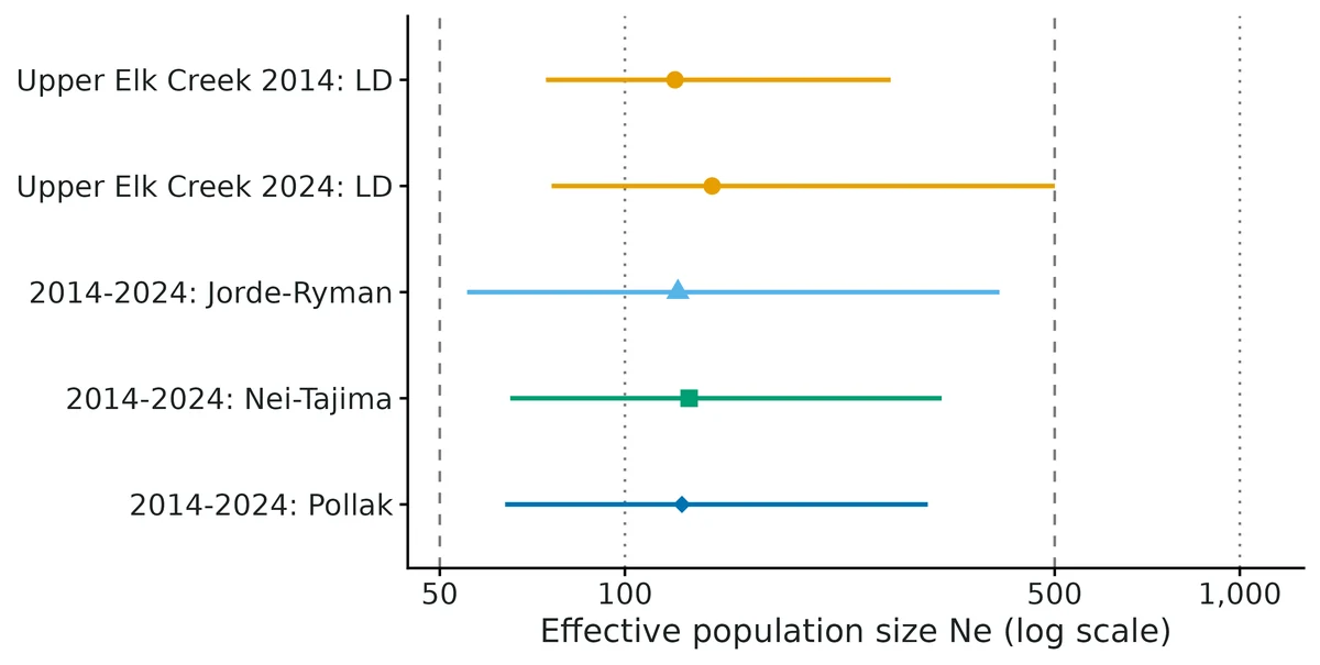
- Temporal method (2014 and 2024, 2.0 generations apart, sampling plan I, census N = 120): Jorde & Ryman's Fs' = 0.0082 gives Ne = 122 (95% CI 55.4 to 407). Nei-Tajima and Pollak estimators give 127 and 124.
- Sample 2014 (50 individuals, 16 loci): the linkage-disequilibrium estimate of Ne is 121 (95% CI 74.4 to 271). An Ne of this size loses about 0.41% of its heterozygosity per generation, about 4.1% over 10 generations, unless immigration or mutation replaces it.
- Sample 2024: the linkage-disequilibrium estimate of Ne is 139 (95% CI 76.0 to 500).
- The interval lies above 50 but reaches below 100: the population passes the classic short-term threshold (50) but not clearly the revised one (100; Frankham et al. 2014).
- Relatedness in sample 2024 (1891 pairs): 15 pairs have r >= 0.354 (likely first-degree) and 86 have 0.177 <= r < 0.354 (likely second-degree); about 7.0% of truly unrelated pairs would be called second-degree or closer; 80% of full sibs and 46% of half sibs fall in their own class.
- Known fullsib pairs (n = 6) have mean r = 0.494 (95% CI 0.296 to 0.693), against a pedigree expectation of 0.50.
- F_IS = 0.028 (95% CI -0.026 to 0.081) in 2014 and 0.004 (-0.025 to 0.032) in 2024: consistent with random mating.
- Ne is not census size; with separate sexes LD estimates ran about 5-25% above the true Ne in validation, whereas the temporal estimate was within 6%; treat a single LD estimate as slightly optimistic.
More figures
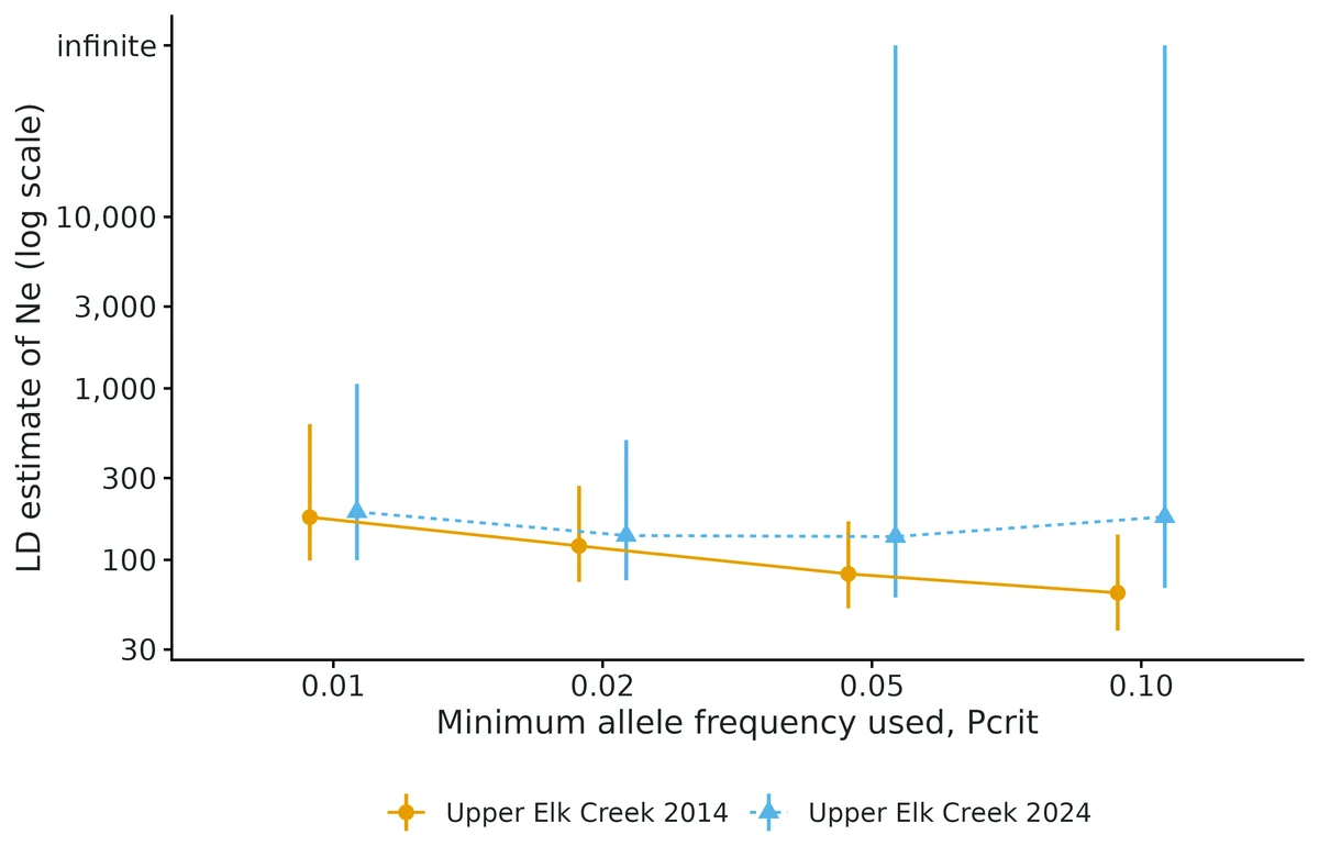
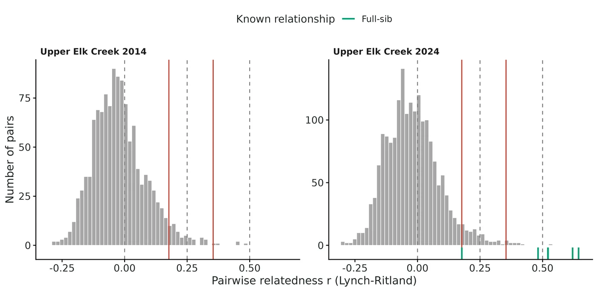
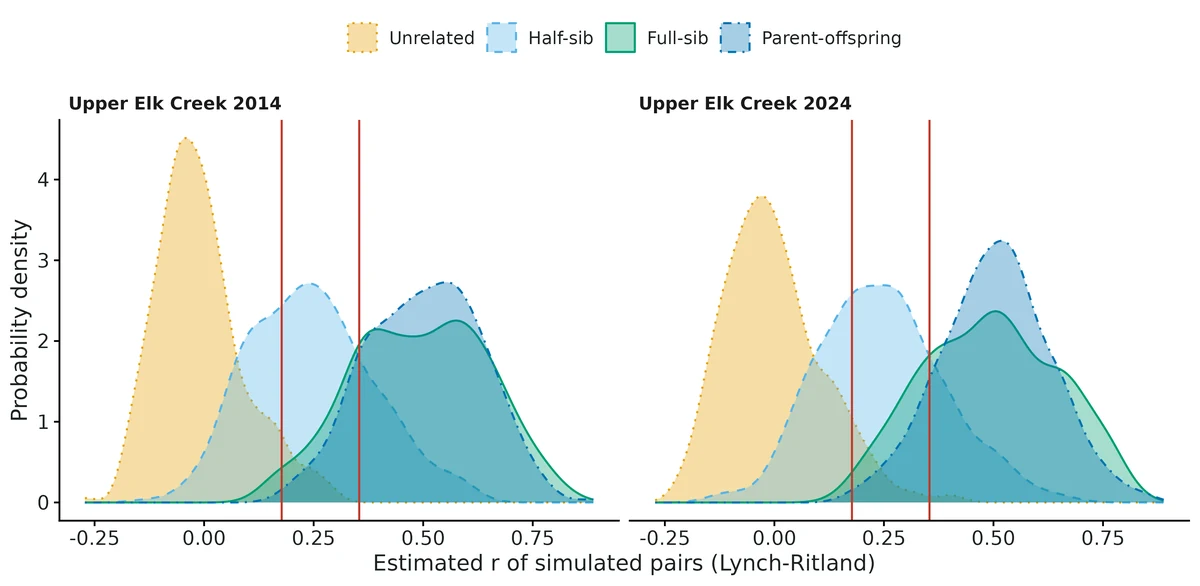
Figures are the module's default publication figures, reduced for the web. The report also saves them as PDF and full-resolution PNG.
Planted truth at the example's design
Before trusting the example's results, the module was run on many simulated data sets with the same design and known true values. Each row is one quantity: did the method get it back? (What the thresholds are.)
What OPEN means here. The module works (it passes at its default design), but at this example's design not every quantity passed the planted-truth check, so CascadiaTools does not certify those. 3 of the 5 quantities checked passed outright. For het loss LD early, het loss LD late, the estimate was biased (by up to 13%); don't interpret those at this design. The quantities that passed can be used as reported. With your own data, the report would say the same and suggest what would help: more data, a simpler model or a different estimator. More on DONE and OPEN.
Why, for this example:
Planted truth at this design: temporal het_loss (+1.6%, coverage 0.92) and full-sib relatedness (LR -2.1%, QG +3.9%) PASS; single-sample LD het_loss FAILS the 10% bias rule in both years (-13.1%, -11.5%; Ne overstated ~15%) because each sample is 42% of the population. Report temporal Ne 122 (55-407) as the answer; LD estimates are supporting, upward-leaning evidence only.
| This example | 16 microsatellites, 50 adults per sample, two samples 2 generations apart, census 120 |
|---|---|
| Design the module was validated at | 1,000 SNPs, 60 individuals per sample, two samples 5 generations apart, Ne 100 |
The example is harder than the validated default: 16 microsatellites instead of 1,000 SNPs, samples only 2 generations apart (the temporal method was validated for 3-10 generations), and each sample is a large share of the population. A hard design with 15 microsatellites and 30 individuals passed the gate but was nearly uninformative (LD upper limit infinite in 93-94% of runs), and the LD method overstated Ne when the sample was a large share of the population or the population had separate sexes (Ne +6% to +25% in independent checks).
These calls sit close to the pass/fail line. With another 200 simulated data sets they could come out the other way, so read them as “about at the limit” rather than as a clear pass or fail.
- het_loss_LD_late (✗ FAIL): bias -11.5% against an allowance of ±10.0% (set by the 10% rule), so it used 115% of the allowance.
3 of 5 rows pass; 1 is borderline.
| Quantity | True value | Average estimate | Bias | Allowed bias | Coverage (needed) | Result |
|---|---|---|---|---|---|---|
| het_loss_LD_early | 0.00417 | 0.00362 | -13.2% | ±10.0% | 0.96 (0.904) | ✗ FAIL |
| het_loss_LD_late | 0.00417 | 0.00369 | -11.5% | ±10.0% | 0.95 (0.904) | ✗ FAIL ≈ borderline |
| het_loss_temporal | 0.00417 | 0.00423 | +1.6% | ±10.2%† | 0.92 (0.904) | ✓ PASS |
| relatedness_fullsib_LR | 0.469 | 0.459 | -2.1% | ±10.0% | 0.97 (0.904) | ✓ PASS |
| relatedness_fullsib_QG | 0.469 | 0.487 | +3.8% | ±10.0% | 0.96 (0.904) | ✓ PASS |
Limits that matter
- LD Ne overstated when the sample is a large share of the population: at S = 50, N = 120 planted-truth LD 1/Ne bias -13%/-12% (gate FAIL).
- LD Ne overstated by 6-25% in separate-sex populations (independent verification); the simulator is monoecious, bull trout are not, so real LD bias may be larger. Temporal method unaffected.
- Overlapping generations not validated: a single-sample LD estimate for bull trout approximates the number of breeders (Nb), not per-generation Ne.
- Temporal method with < 3 generations between samples was outside module validation; this example's own recovery at 2 generations passes (bias +1.6%, coverage 0.92).
- Temporal CI relies on a simulation-calibrated design effect; coverage 0.90-0.92 with 15-20 microsatellites (nominal 0.95).
- With missing microsatellite data, LD Ne differs from NeEstimator by a median 1.7% (max 12%).
- Half-sib misclassification is under-predicted by the simulated-pair table; treat second-degree calls as tentative.
- Not validated: migration/structure, null alleles or genotyping error, selection. The module estimates Ne, never census N.
All known limits from the module's validation record
- LD Ne overestimated in separate-sex populations (independent verification): +6-25% in Ne (1/Ne bias -6% to -20%) with no selfing, worst with 20 microsatellites, skewed sex ratio or S a large share of N; LD coverage 0.76-0.91. The temporal method is unaffected. Monoecious controls pass.
- Ne overestimated when S << Ne. At S = 50 and Ne = 500, LD 1/Ne is biased -6% to -12% (Ne +7-14%; section 3, design grid). With 10 microsatellites and S = 25 the bias is large in either direction (grid: harmonic-mean Ne 39 at Ne 50, 267 at Ne 500). Report the interval, not the point estimate.
- LD jackknife CI is slightly narrow with many SNPs: coverage 0.91-0.93 at the default design (1,000 SNPs), 0.89-0.93 at Ne 500. It passes the gate but is below nominal; the parametric CI is far worse and is not used. At S = 200 the grid used the parametric CI and its coverage with SNPs was 0.20-0.58 (not the module's default; the power run in section 7 uses the jackknife at S = 200).
- Temporal CI relies on a simulation-calibrated design effect (constant 0.5) for correlated frequency change among loci in drift LD. Calibrated and tested only for unlinked loci, Wright-Fisher demography and 3-10 generations. With 15-20 microsatellites coverage is 0.90-0.905 (bound 0.885; nominal 0.95).
- Missing data, microsatellites: our LD estimate differs from NeEstimator's by a median 1.7% (max 12%) in Ne because alleles are screened per locus rather than per locus pair (section 8). Not a bias in recovery, but results will not reproduce NeEstimator to the digit when data are missing.
- Queller-Goodnight for unrelated pairs runs 7-13% more negative than the sample-relative truth (absolute 0.002); Lynch-Ritland (the default
rel_primary) does not. QG passes everywhere except the large-Ne design. - Relatedness CIs for class means are conservative (coverage 0.94-1.00; SE 1.2-1.5x the empirical SD).
- Half-sib misclassification is under-predicted by the simulated-pair table (section 9).
- Not validated: overlapping generations (LD estimates then approximate Nb; Waples et al. 2014), migration/structure, linked SNPs (all simulations use unlinked loci; tightly linked SNPs will bias LD Ne downward), selection, the monogamy mating option, null alleles/genotyping error, the bottleneck test under stepwise mutation, and the temporal method with fewer than 3 generations between samples.
- Simulations use Ne = N (ideal population); the module estimates Ne, never census N.
How this module was validated
- 200 simulated Wright-Fisher populations at the default design (100 for other designs), scored on heterozygosity loss per generation, 1/(2Ne), and relatedness class means; default PASSED all 9 estimands (bias at most 7.3%, coverage 0.910-1.000).
- Harder design (15 microsatellites, 30 per sample, Ne 200, 3 generations, 5% missing) passed all 9 but gave very wide intervals; large Ne (500 with 50 per sample) failed 2 of 9, with Ne overestimated about 13%.
- Negative controls failed as required: wrong sampling plan for the temporal method (-40% bias, coverage 0.04) and full-sib families left in the sample (LD +26%, coverage 0.18).
- False-positive check at effectively infinite Ne: a finite upper Ne limit was claimed in 0/100 (LD) and 5/100 (temporal) replicates.
- Cross-checks: identical to the NeEstimator v2 program on its own worked example, within 0.3% (SNPs) and a median 1.7% (microsatellites with missing data) on 20 simulated sets, and identical to Demerelate for Lynch-Ritland relatedness.
- Design-precision grid and power runs over 25-200 individuals: once there are hundreds of SNPs, individuals rather than loci limit precision; at Ne 500, 25 per sample usually could not bound Ne.
- A separate verifier agent with its own separate-sex simulator found LD Ne biased upward by 6-25% (temporal method unaffected), confirmed the default results exactly, and fixed several silent data-entry problems; verdict: verified with limits.
Every run uses the acceptance gate described on the validation page. The full record follows, section by section, exactly as kept in the module's VALIDATION.md.
Settings and pass/fail rule used for every run
All recovery runs: bin/Rscript core/run.R recover popgen-ne [--config modules/popgen-ne/validation/<cfg>.yaml] --nsim N --cores 16 --out results/popgen-ne/recover_<cfg> (launcher dev/popgen-ne/run_recover_all.sh), 2026-10-19, R 4.5.3, engine as in this folder. Recovery uses fast_settings (no simulated kin pairs, no Pcrit grid, no heterozygosity table; these do not change the estimates that are checked). Replicate r uses seed 100000 + r, so designs that differ only in the fitting or in one design knob share data sets. Gate (core recovery_gate, unchanged): |bias| <= max(10% of truth, 3 MC SE); coverage >= 0.95 - 3 MC SE (floor 0.80); >= 90% of replicates "converged" (here: finite estimates). No threshold was changed.
Simulation model (simulate.R): Wright-Fisher population of N = Ne diploids (random union of gametes, selfing allowed, discrete generations), unlinked loci, founders in HWE/LE, 15 generations of burn-in. An "early" sample of S individuals, a "late" sample S individuals generations_between generations later (non-lethal: sampling plan I, census N known), and a kin panel of full-sib and half-sib pairs born in the late generation (not used for Ne). Kinship is tracked exactly through the pedigree; the relatedness truth for a pair is its pedigree relatedness re-expressed relative to the sampled group (the reference moment estimators use): r* = 2(theta_ij - theta_i. - theta_.j + theta_..)/(1 - theta_..), which is why the full-sib truth is 0.48, not 0.50.
Estimands checked (biological scale): het_loss_LD_<sample> and het_loss_temporal = 1/(2Ne), the proportion of heterozygosity lost per generation (truth 1/(2Ne)). This is the scale on which LDNe and the temporal estimators are nearly unbiased and on which the estimate stays finite when Ne is infinite; Ne itself is reported as 1/(2 het_loss) with the transformed interval. relatedness_<class>_<LR|QG>: mean r of the known pairs of each class.
Verdict
| design | result |
|---|---|
| default (Ne 100, 1,000 SNPs, S = 60 per sample, 5 generations apart; nsim 200) | PASS all 9 estimands |
| hard: 15 microsatellites, S = 30, Ne 200, 3 generations, 5% missing (nsim 100) | PASS all 9 (LD and temporal Ne very imprecise: upper limit infinite in 93-94% / 77% of replicates) |
| large Ne: Ne 500, S = 50, 1,000 SNPs (nsim 100) | 7/9 PASS. FAIL het_loss_LD_late bias -11.9% (MC SE 2.5%), i.e. Ne biased upward ~13% when S << Ne; FAIL relatedness_unrelated_QG -13% of a truth of -0.011 (absolute -0.0014) |
| negative control 1: temporal method told plan II when data are plan I (census N withheld) | FAIL as required: het_loss_temporal -40%, coverage 0.04 |
| negative control 2: 20 full-sib families (40 juveniles) left in the late Ne sample | FAIL as required: het_loss_LD_late +26% (Ne biased down ~21%), coverage 0.18 |
| false-positive rate (Ne = 10,000, effectively no drift signal; nsim 100) | finite upper Ne limit claimed in 0/100 (LD early), 0/100 (LD late), 5/100 (temporal) |
| cross-check vs NeEstimator v2 C program, its own worked example 8Ne50 | LD r^2, Ne, parametric CI: identical (0 relative difference, 40 sample x Pcrit cells); temporal Fk, Fc, Fs, Fs', Ne: identical (16 cells) |
| cross-check vs NeEstimator on 20 simulated data sets with 5% missing genotypes | temporal: <= 5e-4 relative difference (rounding); LD with SNPs: median 0.3% difference in Ne; LD with microsatellites: median 1.7%, max 12% (different missing-data allele screening, see Known limits) |
| cross-check relatedness vs Demerelate 0.9-3 (Lynch-Ritland) | max abs difference 1.1e-16 over 300 pairs |
| bottleneck test size at mutation-drift equilibrium (500 data sets) | 0.052 (MC SE 0.010) with the module's Monte Carlo test; the BOTTLENECK-style Wilcoxon test rejected 0.128 (anti-conservative, now reference only) |
The module is DONE at the default design for LD Ne, temporal Ne and relatedness class means, with the limits below. The large-Ne design (S = 50 with Ne = 500) fails the 10% bias rule for one LD sample; this is a known property of LDNe when the sample is much smaller than Ne (it is in the design grid, section 6) and is reported, not hidden.
Honesty notes.
- The temporal (Jorde-Ryman) CI was changed during validation. The first full run used NeEstimator's normal-approximation jackknife over loci. At the hard design (15 microsatellites) its coverage was 0.88 (bound 0.885: FAIL; 10/12 misses were intervals lying entirely below the truth). It was replaced by a chi-square interval on the uncorrected Fs with df = 2/CV^2 from the same jackknife (the construction NeEstimator uses for the LD jackknife CI), mapped to Fs'. All runs in this file were then repeated with the final engine; first-run outputs are kept in
results/popgen-ne/v1_normalci_*. - With hundreds of SNPs, every published temporal CI is far too narrow because allele-frequency changes at unlinked loci are correlated through drift LD in a small population. At the default design the jackknife SE was 1.6x too small (coverage of the plain jackknife interval about 0.79). The module inflates the jackknife variance by DEFF = 1 + 0.5 (D - D/L) R^2', with D independent alleles, L loci and R^2' the drift LD measured by the LD method in the same samples. The constant 0.5 was chosen on exploration runs (seeds 5001-5120,
dev/popgen-ne/explore_var.R, logs/popgen-ne_explore*.log) and then tested on new seeds (sections 1-3, 5). The same DEFF scales the df of the Nei-Tajima and Pollak chi-square CIs. - The bottleneck test was changed from BOTTLENECK's Wilcoxon signed-rank test to a Monte Carlo test after the size check showed 0.18 (100 data sets) / 0.128 (500) false rejections at equilibrium.
1. Recovery at the default design (nsim 200, 0 errors, median 112 s per replicate on 16 shared cores)
Ne = 100, 1,000 SNPs (MAF 0.05-0.95 in founders), S = 60 per sample, 5 generations between samples, census N = 100 (plan I), 15 full-sib and 15 half-sib pairs, 300 unrelated pairs. results/popgen-ne/recover_default/.
| param | truth | mean est | rel. bias | bias MC SE | coverage (bound) | CI width | mean SE / emp. SD | gate |
|---|---|---|---|---|---|---|---|---|
| het_loss_LD_early | 0.0050 | 0.00483 | -3.4% | 0.9% | 0.910 (0.904) | 0.00231 | 0.94 | PASS |
| het_loss_LD_late | 0.0050 | 0.00483 | -3.4% | 0.8% | 0.930 (0.904) | 0.00224 | 1.00 | PASS |
| het_loss_temporal | 0.0050 | 0.00497 | -0.7% | 0.7% | 0.965 (0.904) | 0.00189 | 1.03 | PASS |
| relatedness_fullsib_LR | 0.4795 | 0.4803 | +0.2% | 0.2% | 0.985 (0.904) | 0.059 | 1.24 | PASS |
| relatedness_fullsib_QG | 0.4795 | 0.4875 | +1.7% | 0.1% | 0.940 (0.904) | 0.055 | 1.23 | PASS |
| relatedness_halfsib_LR | 0.2322 | 0.2306 | -0.7% | 0.3% | 0.995 (0.904) | 0.064 | 1.45 | PASS |
| relatedness_halfsib_QG | 0.2322 | 0.2350 | +1.2% | 0.3% | 0.995 (0.904) | 0.065 | 1.44 | PASS |
| relatedness_unrelated_LR | -0.0266 | -0.0261 | +1.7% | 0.5% | 1.000 (0.904) | 0.013 | 1.32 | PASS |
| relatedness_unrelated_QG | -0.0266 | -0.0285 | -7.3% | 0.9% | 0.985 (0.904) | 0.019 | 1.37 | PASS |
On the Ne scale (dev/popgen-ne/ne_scale_summary.R): LD early/late median Ne 104.6 / 104.4, harmonic mean (1/mean(1/Ne)) 103.5 / 103.5, mean log(Ne_hat/Ne) +0.043 / +0.041; temporal median 100.5, harmonic mean 100.7, mean log ratio +0.011. No infinite estimates or infinite upper limits.
The relatedness class-mean CIs are deliberately conservative (SE = max of the jackknife over loci and over individuals; 1.2-1.5x the empirical SD), because the locus jackknife alone ignores sampling of pairs and the individual jackknife alone ignores locus sampling (exploration: each alone covered 0.70-0.95 depending on class).
2. Harder design (nsim 100, 0 errors)
Ne 200, 15 microsatellites (10 alleles, Dirichlet(1) founder frequencies), S = 30 per sample, 3 generations apart, 5% missing genotypes, 10 full-sib + 10 half-sib pairs. results/popgen-ne/recover_hard_msat/.
| param | truth | mean est | rel. bias | bias MC SE | coverage (bound) | CI width | gate |
|---|---|---|---|---|---|---|---|
| het_loss_LD_early | 0.0025 | 0.00217 | -13.2% | 7.5% | 0.97 (0.885) | 0.0101 | PASS (within 3 MC SE) |
| het_loss_LD_late | 0.0025 | 0.00232 | -7.0% | 8.0% | 0.99 (0.885) | 0.0105 | PASS |
| het_loss_temporal | 0.0025 | 0.00240 | -4.0% | 9.6% | 0.90 (0.885) | 0.0086 | PASS |
| relatedness_fullsib_LR | 0.4755 | 0.4694 | -1.3% | 1.0% | 0.97 | 0.279 | PASS |
| relatedness_fullsib_QG | 0.4755 | 0.4914 | +3.3% | 0.9% | 0.99 | 0.243 | PASS |
| relatedness_halfsib_LR | 0.2294 | 0.2137 | -6.8% | 1.6% | 1.00 | 0.246 | PASS |
| relatedness_halfsib_QG | 0.2294 | 0.2347 | +2.3% | 1.6% | 0.99 | 0.250 | PASS |
| relatedness_unrelated_LR | -0.0208 | -0.0214 | -2.7% | 3.2% | 0.98 | 0.038 | PASS |
| relatedness_unrelated_QG | -0.0208 | -0.0232 | -12.2% | 6.3% | 0.98 | 0.067 | PASS |
The gate passes, but the design is nearly uninformative about Ne: the LD estimate was infinite in 12-13% of replicates and its upper limit infinite in 93-94%; the temporal upper limit was infinite in 77%. Median LD Ne 225 / 222 (truth 200), mean log ratio of finite estimates +0.34 / +0.19. Read: with 15 microsatellites and 30 individuals per sample the interval nearly always reaches infinity, so such data can at most give a lower bound for Ne.
3. Large Ne relative to the sample (nsim 100)
Ne 500, S = 50, 1,000 SNPs, 5 generations. results/popgen-ne/recover_large_ne/.
| param | truth | mean est | rel. bias | bias MC SE | coverage | gate |
|---|---|---|---|---|---|---|
| het_loss_LD_early | 0.0010 | 0.000939 | -6.1% | 2.7% | 0.93 | PASS |
| het_loss_LD_late | 0.0010 | 0.000881 | -11.9% | 2.5% | 0.89 | FAIL (bias) |
| het_loss_temporal | 0.0010 | 0.000943 | -5.7% | 2.5% | 0.93 | PASS |
| relatedness LR (3 classes) | -0.2% to +0.8% | 0.99-1.00 | PASS | |||
| relatedness QG full/half sib | +1.2% to +1.5% | 0.95-0.99 | PASS | |||
| relatedness_unrelated_QG | -0.0112 | -0.0127 | -13.3% | 3.0% | 0.97 | FAIL (bias; absolute -0.0014) |
On the Ne scale: LD median 515 / 593, harmonic mean 532 / 567 (truth 500), mean log ratio +0.12 / +0.17. Both LD samples err in the same direction (pooled -9%), and the design grid (section 6) shows the same pattern (-5% to -12% in 1/Ne at S = 50, Ne = 500). LDNe's sample-size correction slightly over-subtracts when S is much smaller than Ne, so Ne is overestimated by roughly 10-15% when S is about Ne/10. This is reported in the interpretation via the design figure and in Known limits.
4. Negative controls (the gate can fail)
Both share seeds with the default design (identical early samples).
Mis-specified sampling plan (validation/misspec_plan2.yaml): data simulated under plan I (sampled individuals return and reproduce, census N = 100), but the census size is withheld, so the temporal method applies the plan II correction. het_loss_temporal: mean 0.00298 vs truth 0.005 (-40%), coverage 0.04 -> FAIL. LD and relatedness unaffected (PASS; het_loss_LD_early coverage 0.88 on these 100 replicates, just below 0.885; the same data at nsim 200 in section 1 give 0.91).
Family over-representation (validation/misspec_sibs.yaml): 20 full-sib pairs (40 juveniles of 20 families) are added to the late sample and used for Ne (use_for_ne not set). het_loss_LD_late +26.3% (Ne -21%), coverage 0.18 -> FAIL. The temporal estimate is barely affected (+3.4%, coverage 0.95). This is the Waples & Anderson (2017) situation; the module's use_for_ne column exists to avoid it.
5. False-positive rate (no drift signal)
validation/null_infinite.yaml: Ne = 10,000 (het_loss = 0.00005), S = 60, 1,000 SNPs. The relevant error is claiming a finite upper limit for Ne (CI for het_loss excluding 0 from above): 0/100 for LD early, 0/100 for LD late, 5/100 for temporal (nominal 0.025 one-sided, 0.05 two-sided; MC SE 0.022). Intervals entirely below 0 (no evidence of drift at all) occurred in 4/100 and 2/100 LD replicates. LD point estimates were infinite in 46-51% of replicates, as expected. The bias gate "fails" here (-73% / -81% of 0.00005, absolute -0.00004 in het_loss, i.e. a 0.1% error in E(r^2_sample)); it is irrelevant at this Ne and reported for completeness.
6. Design precision: individuals and loci needed
40 replicates per cell; LD method on one sample; CV = RMSE(1/Ne_hat)/(1/Ne). Jackknife CIs for S <= 100; parametric CIs for S = 200 (speed), which is why coverage collapses there (see Known limits).
| Ne | S | 500 SNPs CV | 2,000 SNPs CV | 10 msats CV | 20 msats CV | P(upper = inf), 20 msats |
|---|---|---|---|---|---|---|
| 50 | 25 | 0.22 | 0.21 | 0.78 | 0.53 | 0.15 |
| 50 | 50 | 0.11 | 0.10 | 0.31 | 0.22 | 0 |
| 100 | 25 | 0.28 | 0.21 | 0.88 | 0.45 | 0.40 |
| 100 | 50 | 0.13 | 0.12 | 0.48 | 0.23 | 0 |
| 100 | 100 | 0.08 | 0.06 | 0.18 | 0.14 | 0 |
| 500 | 25 | 0.66 | 0.49 | 2.41 | 1.39 | 0.95 |
| 500 | 50 | 0.27 | 0.19 | 1.14 | 0.51 | 0.78 |
| 500 | 100 | 0.13 | 0.13 | 0.65 | 0.27 | 0.23 |
| 500 | 200 | 0.08 | 0.07 | 0.29 | 0.12 | 0 |
Harmonic-mean Ne over replicates (1/mean(1/Ne_hat)) is within 15% of the truth in every SNP cell (worst: 435 at Ne 500, S 25, 500 SNPs; 570 at Ne 500, S 50, 500 SNPs); with 10 microsatellites and S = 25 it ranges from 39 (Ne 50) to 267 (Ne 500). Rules of thumb from the grid: for CV <= 0.2, Ne = 50 needs S ~ 50 with 500+ SNPs (CV 0.10-0.11; 20 microsatellites give 0.22); Ne = 100 needs S ~ 50 SNPs-wise or S ~ 100 with 20 microsatellites; Ne = 500 needs S ~ 100 with SNPs or S ~ 200 with 20 microsatellites. More SNPs beyond ~500 help little: individuals, not loci, limit precision once there are hundreds of SNPs. The design_precision figure in every report shows this grid with the study's S marked.
7. Power over sample size
bin/Rscript core/run.R power popgen-ne --config modules/popgen-ne/validation/large_ne.yaml --vary n_ind=25,50,100,200 --nsim 50 --cores 16 --out results/popgen-ne/power_nind (Ne = 500, 1,000 SNPs, 5 generations). "Power" = share of replicates whose CI for het_loss excludes 0, i.e. that give a finite upper limit for Ne.
Run 2026-10-19 with the final engine; results/popgen-ne/power_nind/. CV = RMSE / truth on the het_loss (1/(2Ne)) scale. Coverage MC SE at nsim 50 is about 0.03.
| S per sample | estimand | power (finite upper Ne limit) | rel. bias | CV | coverage |
|---|---|---|---|---|---|
| 25 | LD early | 0.32 | +6.0% | 0.51 | 0.96 |
| 25 | LD late | 0.40 | +6.8% | 0.48 | 0.92 |
| 25 | temporal | 0.74 | +3.6% | 0.42 | 0.96 |
| 50 | LD early | 0.96 | -9.9% | 0.31 | 0.88 |
| 50 | LD late | 1.00 | -3.5% | 0.24 | 0.94 |
| 50 | temporal | 1.00 | +1.9% | 0.28 | 0.90 |
| 100 | LD early | 1.00 | -2.7% | 0.13 | 0.96 |
| 100 | LD late | 1.00 | +0.4% | 0.12 | 0.98 |
| 100 | temporal | 1.00 | +1.0% | 0.13 | 0.96 |
| 200 | LD early | 1.00 | -2.1% | 0.08 | 0.94 |
| 200 | LD late | 1.00 | -2.8% | 0.07 | 0.98 |
| 200 | temporal | 1.00 | -0.2% | 0.08 | 0.98 |
Read: at Ne = 500 with 1,000 SNPs, 25 individuals per sample usually cannot bound Ne from above (LD 32-40%); 50 individuals almost always can but with CV 0.24-0.31; 100 individuals give CV ~0.13 and 200 give ~0.08. This matches the design grid (section 6). The S = 50 LD-early cell repeats the downward 1/Ne bias (Ne too high) of section 3; at S >= 100 the bias is <= 3%.
8. Cross-checks against independent implementations
NeEstimator v2 (C source, compiled; dev/popgen-ne/neestimator/, SOURCE.txt). (a) Its distributed worked example 8Ne50 (8 samples x 50 individuals, 20 microsatellites, true Ne 50), 5 Pcrit settings (dev/popgen-ne/crosscheck_example.R, results/popgen-ne/validation/crosscheck_8Ne50_*.csv): LD r^2, E(r^2), Ne and parametric CI identical to all printed digits (40/40 cells); jackknife-on-samples CI within 2.2% (lower) and 3.9% (upper), largest in the singleton-only ("No S*") column where NeEstimator re-screens alleles per locus pair. Temporal (samples paired as generations 0 and 1.5, plan II): Fk, Fc, Fs, Fs', Jorde-Ryman Ne and its jackknife CI identical (16/16 cells). The worked example's LD estimates (45-87 across samples and Pcrit, true 50) are themselves a check of the method against a known-truth published data set. (b) 20 simulated data sets (10 with 15 microsatellites, 10 with 300 SNPs; S = 50/60; 5% missing genotypes; plan I, census 100; dev/popgen-ne/crosscheck_sims.R, crosscheck_sims_neestimator.csv):
| quantity | marker | median / max relative difference: r^2 or Fs | Ne | CI lower | CI upper |
|---|---|---|---|---|---|
| LD early | msat | 0.18% / 0.59% | 1.6% / 8.3% | 1.7% / 2.6% | 6.6% / 13% |
| LD late | msat | 0.20% / 1.2% | 1.8% / 12% | 2.0% / 7.4% | 4.8% / (one infinite vs finite) |
| LD early | SNP | 0.04% / 0.13% | 0.3% / 1.0% | 0.3% / 0.8% | 0.6% / 1.5% |
| LD late | SNP | 0.04% / 0.09% | 0.3% / 0.8% | 0.4% / 0.8% | 0.3% / 1.2% |
| temporal JR | msat | 0.01% / 0.02% | 0.02% / 0.05% | 0.04% / 0.08% | 0.01% / 0.04% |
| temporal JR | SNP | 0.01% / 0.02% | 0.02% / 0.05% | 0.04% / 0.06% | 0.02% / 0.04% |
(The temporal comparison uses NeEstimator's normal jackknife interval, which the module keeps internally as Fp_lo_normal/Fp_hi_normal, without the design effect.) The LD differences with missing data come from one documented choice: NeEstimator recomputes allele frequencies, the Pcrit screen and the number of independent alleles separately for every locus pair from the individuals typed at both loci, whereas this module screens alleles once per locus over all typed individuals and computes each pairwise r^2 from pairwise-complete moments. With complete data the two are identical (8Ne50). Recovery with 5% missing data (section 2) shows no bias attributable to this choice.
Relatedness (dev/popgen-ne/crosscheck_rel.R, 15 microsatellites, 300 pairs): Lynch-Ritland identical to Demerelate 0.9-3's lxy/lxy.w (max |difference| 1.1e-16). Queller-Goodnight: identical to a direct loop over the QG (1989) ratio-of-sums formula (3.3e-16); Demerelate's rxy averages per-locus ratios instead (a different estimator; correlation 0.953 with ours). Against an independent estimator family, hierfstat's Weir-Goudet beta (2 x beta.dosage), class means on one data set were full sibs 0.45 (QG 0.42, LR 0.29), half sibs 0.23 (0.21, 0.20), unrelated -0.034 (-0.043, -0.034), pedigree truth 0.47 / 0.23 / -0.021. The low LR full-sib mean on this single data set is estimator noise (LR is the noisiest with highly polymorphic loci): over 100 replicates of the hard design LR full-sib bias was -1.3%.
Analytic expectation. At drift-LD equilibrium E(r^2_drift) ~ 1/(3Ne) for unlinked loci (Hill 1981, the basis of Waples 2006): mean R^2' in the exploration runs was 0.0032 at Ne 100 (1/(3Ne) = 0.0033), 0.0016 at Ne 200 (0.0017), 0.0061 at Ne 50 (0.0067) and 0.00064 at Ne 500 (0.00067).
9. Close-kin calls
Share of pedigree-known pairs called first-degree (r_LR >= 0.354), second-degree (0.177-0.354) or unrelated, observed vs predicted by the module's simulated-pair table (rel_sim_pairs, the source of the report's misclassification sentence):
| panel | class | obs first / second / unrel | predicted first / second / unrel |
|---|---|---|---|
| 1,000 SNPs | full sib | 1.00 / 0 / 0 | 1.00 / 0 / 0 |
| 1,000 SNPs | half sib | 0.01 / 0.88 / 0.10 | 0.01 / 0.97 / 0.02 |
| 1,000 SNPs | unrelated | 0 / 0 / 1.00 | 0 / 0 / 1.00 |
| 300 SNPs | full sib | 0.98 / 0.02 / 0 | 0.99 / 0.01 / 0 |
| 300 SNPs | half sib | 0.04 / 0.75 / 0.21 | 0.06 / 0.81 / 0.13 |
| 300 SNPs | unrelated | 0 / 0.001 / 1.00 | 0 / 0.003 / 1.00 |
| 15 msats | full sib | 0.77 / 0.20 / 0.03 | 0.81 / 0.16 / 0.02 |
| 15 msats | half sib | 0.20 / 0.40 / 0.40 | 0.24 / 0.42 / 0.34 |
| 15 msats | unrelated | 0.002 / 0.038 / 0.96 | 0.006 / 0.063 / 0.93 |
Full-sib and unrelated calls are predicted well (the prediction is slightly pessimistic for unrelated pairs). Half sibs are missed more often than predicted (10% vs 2% with 1,000 SNPs) because real half sibs in a small population score r* ~ 0.23, not 0.25, relative to the sample; the report says so.
10. Bottleneck test
15 loci, 50 individuals, infinite-alleles data generated by the Hoppe urn (theta = 5). Rejection rate at P < 0.05: equilibrium 0.052 (500 data sets; MC SE 0.010); after 4 generations at Nb = 10 or Nb = 25 from an equilibrium population of 1,000: 1.00 and 1.00 (100 each). The Wilcoxon signed-rank test used by BOTTLENECK (Piry et al. 1999) rejected 0.128 at equilibrium, because He given k is skewed; the module reports it only for reference. Not checked: stepwise-mutation data (the test is known to be anti-conservative for microsatellites evolving by SMM under the IAM null).
Independent verification (2026-10-19, separate verifier agent)
Verdict: VERIFIED_WITH_LIMITS. The module recovers truth at the builder's default design (rerun reproduced exactly). It passes the gate for the temporal method and relatedness at independent designs. LD Ne is biased upward in dioecious (separate-sex) populations, which the builder's monoecious simulator could not reveal. The issue is documented in the report text and Known limits below.
Literature / code check. I compared the engine line by line with Waples (2006) / Waples & Do (2008), as implemented in strataG ldNe.R (fetched). E(r^2_sample) = 1/S + 3.19/S^2 (S >= 30) and 0.0018 + 0.907/S + 4.44/S^2. Ne = (a + sqrt(a^2 - b r'))/(2r') with (a, b) = (1/3, 2.76) or (0.308, 2.08). Monogamy uses (2/3, 7.2) and (0.618, 5.24). All are identical in engine.R (exp_r2_sample, ld_inv_ne). Jorde & Ryman (2007) Fs' with the plan I census terms, Ne = t/(2Fs'), and Nei-Tajima Fc / Pollak Fk also match (the builder also matches the NeEstimator C program exactly on 8Ne50). simulate() shares no code with fit() beyond the data structure. The independent simulator below shares none at all.
Default-design rerun (core/run.R recover popgen-ne --nsim 200, results/popgen-ne/verify_rerun_default/): every number in section 1 reproduced to the printed digit. After my fixes, 16 replicates of the default design (results/popgen-ne/verify_postfix16/) give estimates and limits identical to the original run (144/144 rows, max |difference| 0).
Independent planted truth (dev/popgen-ne/verify/verify_sim.R; my own Wright-Fisher simulator, no module code). Design: dioecious population with fixed numbers of males (Nm) and females (Nf), no selfing, truth Ne = 4NmNf/(Nm+Nf) != census N. Other settings: sampling plan I with census N supplied; times in years with generation_time 3; sample labels not "early"/"late"; kin panel; truth for relatedness re-derived from my own kinship recursion. Seeds 777000 + r. Results in results/popgen-ne/verify/, logs in logs/popgen-ne_verify_*.log.
| design | n | het_loss LD (sample 1 / 2): rel. bias, coverage | het_loss temporal | relatedness (6 estimands) |
|---|---|---|---|---|
| A: 600 SNPs, Nm 25 / Nf 75 (Ne 75, N 100), S 40, 4 gen, 3% missing | 150 | -8.9% / -9.8%, cov 0.85 / 0.83 (bound 0.897): FAIL coverage | -0.04%, cov 0.93: PASS | all PASS (QG unrelated -7.9%) |
| B: 20 msats (12 alleles), Nm 15 / Nf 45 (Ne 45, N 60), S 40, 6 gen | 150 | -14.6% / -15.8%: FAIL bias, cov 0.85 / 0.91 | -5.6%, cov 0.93: PASS | 5/6 PASS; QG unrelated -12.8% FAIL (known limit) |
| A_eq: as A, Nm 38 / Nf 37 | 150 | -8.0% / -6.0%, cov 0.89 (FAIL, bound 0.897) / 0.91 | -1.2%: PASS | all PASS |
| A_mono: as A, monoecious with selfing (Ne = N = 75) | 150 | -2.3% / -1.2%, cov 0.96 / 0.97: PASS | +1.3%: PASS | 5/6 PASS (QG unrel -10.4%) |
| B_eq: as B, Nm 30 / Nf 30 | 100 | -11.0% (FAIL) / -8.6% | -1.4%: PASS | QG unrel FAIL |
| B_mono: as B, monoecious, N 60 | 150 | -5.5% / -8.6%: PASS | -2.5%: PASS | all PASS |
| B_eqbig: as B_eq, N 300 (S/N 0.13) | 100 | -9.6% / -13.2% (FAIL bias) | -3.8%: PASS | QG unrel FAIL |
| B_skewbig: Nm 12 / Nf 588 (Ne 47, N 600) | 100 | -17.8% / -20.2%, cov 0.81 / 0.76: FAIL | -5.4%, cov 0.91: PASS | LR half-sib -13.7% FAIL |
On the Ne scale (harmonic mean over replicates): A LD 82-83 vs 75; B LD 53-54 vs 45; B_skewbig 57-59 vs 47; temporal 75.0 (A), 47.7 (B), 49.7 (skewbig). Reading: with separate sexes, the LD estimate overstates Ne by about 6-25%. The bias is largest with few microsatellites, a strongly skewed sex ratio, or a sample that is a large share of the population. The same data run monoecious (A_mono, B_mono) pass, so the cause is the mating system, not a coding error. Waples' (2006) constants were calibrated on random-union-of-gametes (selfing allowed) populations. The temporal method's truth is recovered in every design, which also confirms the simulator's Ne. The pedigree-relative relatedness truth is recovered for LR and QG except the known QG-unrelated limit. LR half sibs are -14% with Nm 12 (inbred background).
Controls.
- Negative control (generation_time given as half the true value, i.e. the generations between samples are wrong) fails as required: temporal bias -49% to -53% in every design, coverage 0-0.52.
- False positives: design N, an infinite population (no drift; 600 SNPs, S 40 x 2, plan II, nsim 200). A finite upper Ne limit (CI for het_loss above 0) was claimed in 0/200 (LD sample 1), 0/200 (LD sample 2) and 4/200 (temporal, 0.02). Two-sided rejection of het_loss = 0 occurred in 0.05 / 0.02 / 0.05 (nominal 0.05). LD point estimates were biased slightly negative (-3e-5, about 0.1% of E(r^2_sample)), harmless.
Usability (messy data, dev/popgen-ne/verify/messy/). Before the fixes:
- A capitalised
Yearcolumn was reported clearly. - A misspelled id column gave "arguments imply differing number of rows: 0, 112".
- A misspelled first locus column gave "NA/NaN argument".
- A typo "2O14" in the year column silently became NA.
- A stray "Yes" in an allele column was silently accepted: the whole locus was recoded as rank codes, giving wrong genotypes with no message.
- A one-fish year typo (2104) became the "late" sample of the temporal method (18 generations, one individual).
- A misspelled site became a separate population with no hint.
Fixes in io.R / module.R:
- Named-column checks that list the actual columns and say names are case-sensitive.
- Non-numeric year values are rejected, naming the individual.
- Non-numeric junk in allele-size columns is rejected, naming the locus and individual.
- Small samples (< 10) are listed with their IDs and a "possibly a misspelling of X?" hint.
- check_data reports individuals with no sampling time.
- The temporal method uses only time points with >= 10 individuals and says which were skipped.
Re-tested: each case now stops or warns with a specific, actionable message. With a blank year, the 2104 typo and a misspelled site in one file, the fit uses 2014 vs 2024 correctly. Estimates on clean data are unchanged (above).
Report and figures (example config, results/popgen-ne/verify_example/). I checked every interpretation sentence against the estimates table:
- het loss 0.41% / 0.36% per generation and 4.1% / 3.5% over 10 generations.
- Thresholds wording.
- Fs' 0.0082 -> Ne 122 over 2 generations.
- 1225 / 1891 pairs; 5.7% x 1225 ~ 69 false calls.
- F_IS statements.
All are correct, with no causal language. The response scale (Ne, proportion of heterozygosity) is stated. All 6 required figures are present and their plotted values match fit$estimates. Changes:
- The Pollak marker was a thin yellow "+" (nearly invisible); all methods now use solid shapes.
- The "inf" axis label now reads "infinite".
- The report's caveat paragraph now states the separate-sexes LD bias.
Changed files: io.R, module.R (temporal time-point filter), output.R (figure shapes/labels, caveat sentence). Originals are in dev/popgen-ne/verify/*.orig. No gate thresholds or core files were changed.
Engine, references and full details
Engine: R implementation of the NeEstimator v2 formulas (LDNe with jackknife CIs; temporal Jorde-Ryman, Nei-Tajima, Pollak), Queller-Goodnight and Lynch-Ritland moment estimators; cross-checked against the NeEstimator C program.
References
Waples 2006; Waples & Do 2008, 2010; Peel et al. 2013; Do et al. 2014 (NeEstimator v2); Jones, Ovenden & Wang 2016; Nei & Tajima 1981; Pollak 1983; Waples 1989; Jorde & Ryman 2007; Queller & Goodnight 1989; Lynch & Ritland 1999; Wang 2014; Manichaikul et al. 2010; Cornuet & Luikart 1996; Piry et al. 1999; Franklin 1980; Frankham et al. 2014; Franklin, Allendorf & Jamieson 2014; Frankham 1995; Waples & England 2011; Waples, Antao & Luikart 2014; Waples & Anderson 2017. Full citations in module.R (references).
