Demography and population dynamics

Population viability analysis - count-based (diffusion / state-space) and matrix-model PVA

"How likely is this population to drop to a level we would consider functionally extinct (the quasi-extinction threshold) within the next 10, 25 or 50 years; how fast is it growing or declining in the long run; and which vital rates, or which management actions, would most reduce the risk?"

module id: pva! Example verdict: OPEN6 of 7 quantities certified

Is this the right analysis?

Use it when

The question is extinction or quasi-extinction RISK - "how likely is this population to fall below N animals within 10, 25 or 50 years, and which vital rates or management actions change that?" Use the count model when you have one count or index per year (10+ years, ideally 20+). Use the matrix model when you have stage- or age-specific vital rates (survival, fecundity) with standard errors and year-to-year variation, e.g. from a CJS, IPM or nest-monitoring analysis, or raw annual monitoring counts of animals at risk and survivors / young produced.

Not for

Estimating trend, density dependence or covariate effects on growth from counts (use timeseries, which this module complements); estimating survival from capture histories (cjs / multistate / ipm first, then feed their estimates here); spatially explicit or metapopulation PVA (not supported); fewer than ~10 counts (risk is unestimable); populations with strong density dependence near carrying capacity in the count model (see Pitfalls).

The data you need

Count model - CSV with one row per year (year, count; blank = not surveyed). matrix model - a matrix definition (stages, entries as formulas in named vital rates) in the config plus EITHER a vital-rate CSV (rate, type, mean, se, sd_env, n_years) OR an annual monitoring CSV (year, rate, n, events); initial abundance per stage; a quasi-extinction threshold..

What the example's main data file looks like:

First 5 of 30 rows of `shorebird_breeding_pairs.csv`.
survey_year	breeding_pairs	observer_notes
1994	412
1995	350
1996	430
1997		no survey
1998	499

Not sure? Use the finder to compare modules.

Try it

The worked example

Shorebird breeding-pair survey: count-based state-space PVA with counting error and missing years (simulated)

The question: Is the shorebird population really declining, and how likely is it to fall to 40 breeding pairs or fewer within 10 and 25 years?

The data are simulated, so the true answer is known and the analysis can be checked against it.

What the researcher typed

I have 30 years of spring counts of breeding pairs for a shorebird (shorebird_breeding_pairs.csv; blank = no survey). The counts are surveys, so they're not exact. Please tell me whether the population is declining and how likely it is to drop to 40 breeding pairs or fewer within 10 and 25 years. I don't code, so please do the analysis and give me a report and figures I can use.

Run it yourself

Download the example data below and unzip it.
Open the unzipped folder in Claude Code (see Install).
Paste the prompt above. The agent checks the files, writes a plan, runs planted truth, fits the model and writes the report. You can compare your results with the ones below.

Download the example data (zip, 8 KB)

Contains shorebird_breeding_pairs.csv, the settings file (config_state_space.yaml), a description of the data and a step-by-step walkthrough.

Study design details

model	count
method	state_space
years spanned	30
years surveyed	25
years missing	1997, 2003, 2004, 2011, 2020
first year	1994
N0	420
threshold	40
horizons	10, 25

What the report says

Results from the example data

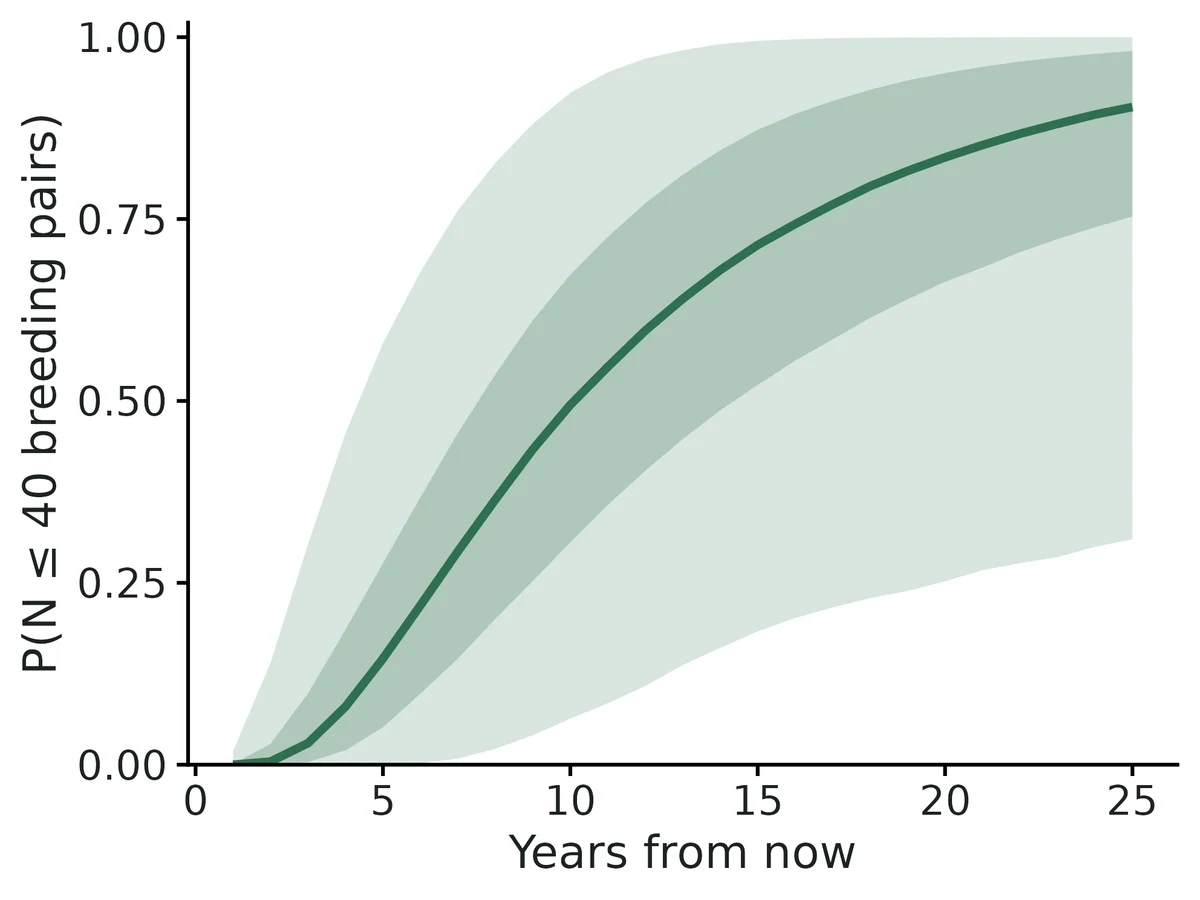
Figure: Cumulative probability that abundance falls to or below the quasi-extinction threshold (40 breeding pairs) by each year. — Cumulative probability that abundance falls to or below the quasi-extinction threshold (40 breeding pairs) by each year. Line: estimate; dark band: 50% and light band: 95% credible interval (posterior of growth rate, variance and current abundance).

What this means

the population was not clearly increasing or decreasing: the long-run (median) growth rate is lambda = 0.942 per year (95% CI 0.879 to 1.013), i.e. a typical change of -5.8% per year (95% CI -12.1% to +1.3%).
Year-to-year variability in the log growth rate (process variance sigma^2) is 0.0188 (95% CI 0.0030 to 0.0971).
Counting (observation) error variance on the log scale is 0.0256 (95% CI 0.0003 to 0.0727), equivalent to a coefficient of variation of roughly 16% in a single count. The model's estimate of the true current abundance is 79 breeding pairs (95% CI 61 to 100).
Probability that the population falls to or below the quasi-extinction threshold of 40 breeding pairs in at least one annual census within 10 years: 49% (95% CI 6% to 92%); 25 years: 90% (95% CI 31% to >99.9%).
Forecasts beyond about 20% of the monitoring span (here 6 years) are known to be very imprecise (Fieberg & Ellner 2000); use them to compare options, not as absolute predictions.

More figures

Figure: Observed counts (points), state-space estimate of true abundance with 95% band (grey) and projected abundance: median (line), 50% and 95% of simulated futures (bands) including uncertainty in growth rate and variance. — Observed counts (points), state-space estimate of true abundance with 95% band (grey) and projected abundance: median (line), 50% and 95% of simulated futures (bands) including uncertainty in growth rate and variance. Dashed line: quasi-extinction threshold.

Figure: Posterior distribution of the long-run growth rate. — Posterior distribution of the long-run growth rate. Solid line: estimate; dashed line: lambda = 1 (stable). Share of posterior draws below 1: 96%.

Figure: Model checks. — Model checks. A: annual log growth rates (per year of interval) with the estimated mu; no trend or strong autocorrelation expected (lag-1 r = -0.31). B: growth rate against log abundance; a clear negative slope (here -0.012, p = 0.874) suggests density dependence, which this model ignores.

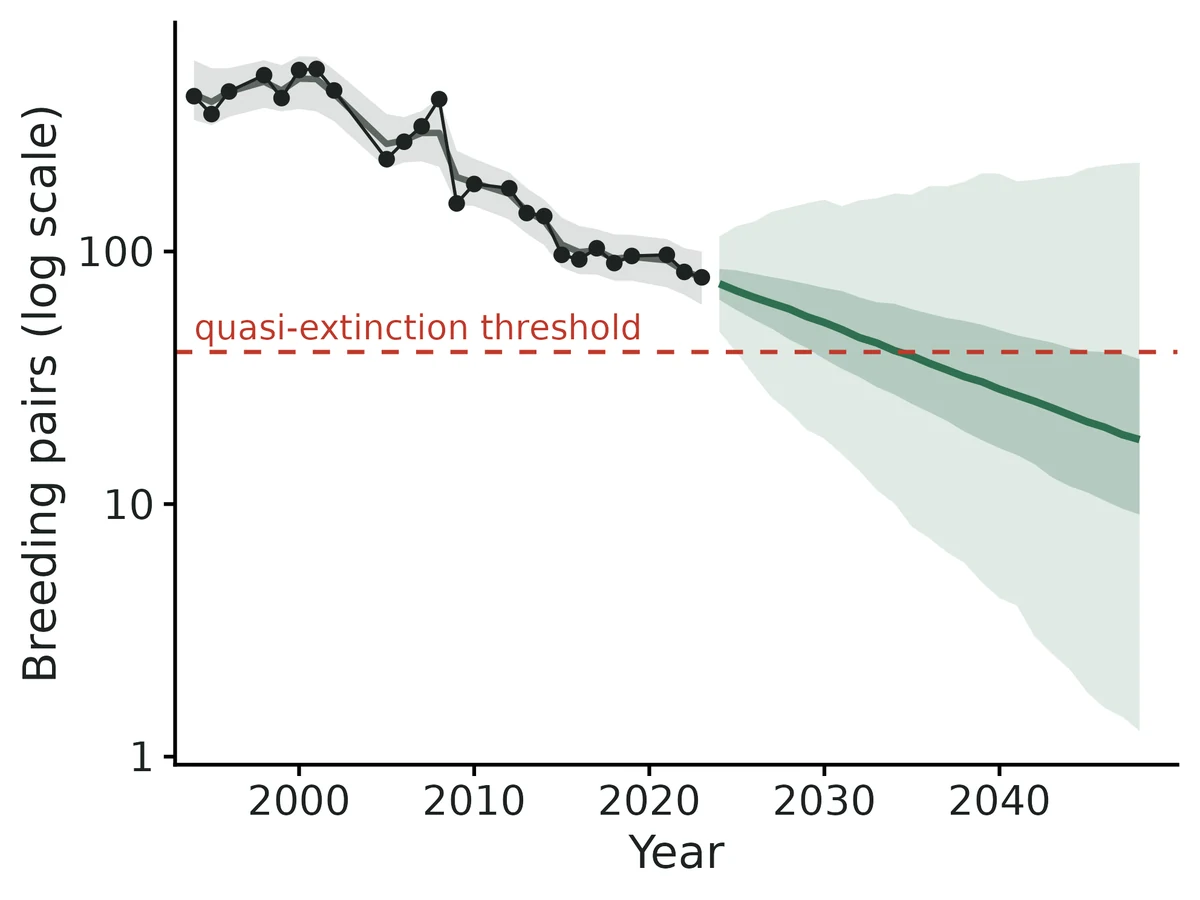
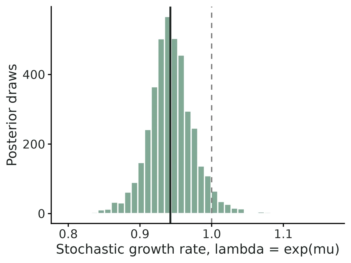
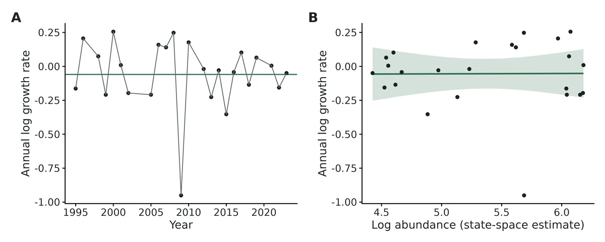
Figures are the module's default publication figures, reduced for the web. The report also saves them as PDF and full-resolution PNG.

How we know it works

Planted truth at the example's design

Before trusting the example's results, the module was run on many simulated data sets with the same design and known true values. Each row is one quantity: did the method get it back? (What the thresholds are.)

Verdict for this example: ! OPEN

What OPEN means here. The module works (it passes at its default design), but at this example's design not every quantity passed the planted-truth check, so CascadiaTools does not certify those. 6 of the 7 quantities checked passed outright. For p qext 10yr, the estimate was biased (by up to 47%); don't interpret those at this design. The quantities that passed can be used as reported. With your own data, the report would say the same and suggest what would help: more data, a simpler model or a different estimator. More on DONE and OPEN.

Why, for this example:

Growth, variances and current abundance pass planted truth and the fit is healthy, but the quasi-extinction point estimate (a primary estimand) fails the mean-bias gate at 10 years (Known limit 1); intervals are calibrated (coverage 0.985), so risk is reported as an interval only.

The example's design compared with the validated design: harder than validated

This example	25 counts over 30 years (5 years missing), state-space count PVA, counting error larger than process noise
Design the module was validated at	25 annual counts with 10% of years missing, state-space count model, counting and process variance both 0.02

The example spans more years than the validated state-space default, but its counting error is larger than its process noise (0.03 against 0.012), as in the harder designs tested. At those designs growth rate, process variance and current abundance passed. Quasi-extinction point estimates failed the mean-bias test at every design (for example +0.074 at 10 years in the default state-space run), although their intervals were calibrated (coverage 0.975-0.98). In a short, gappy series where counting error exceeded process noise, observation variance was also 18% low.

6 of 7 rows pass.

Bias: average estimate minus truth, as a percentage of the truth. Allowed bias: the largest bias that still passes, the bigger of 10% of the truth and 3 Monte Carlo standard errors († = set by that simulation-noise floor, so the allowance is wider than 10%). Coverage: share of 95% intervals that contained the true value, with the minimum needed in brackets. ≈ borderline: the bias used 80–125% of its allowance, or coverage was within 0.015 of the minimum; such a result could flip between PASS and FAIL with another set of simulations. Quantity names are as they appear in the report.
Quantity	True value	Average estimate	Bias	Allowed bias	Coverage (needed)	Result
growth_rate_mu	-0.04	-0.0415	-3.8%	±11.6%^†	0.97 (0.904)	✓ PASS
lambda_stochastic	0.961	0.96	-0.1%	±10.0%	0.97 (0.904)	✓ PASS
N_current	149.5	150.2	+0.5%	±10.0%	0.94 (0.904)	✓ PASS
obs_variance_tau2	0.03	0.0288	-4.0%	±10.3%^†	0.97 (0.904)	✓ PASS
p_qext_10yr	0.162	0.238	+47.0%	±17.6%^†	0.98 (0.904)	✗ FAIL
p_qext_25yr	0.463	0.492	+6.2%	±10.0%	0.98 (0.904)	✓ PASS
process_variance_sigma2	0.012	0.014	+16.7%	±21.8%^†	0.98 (0.904)	✓ PASS

Limits that matter

Quasi-extinction point estimates are median-unbiased but too extreme on average and fail the mean-bias gate; quote the interval (Known limit 1).
Risk horizons beyond ~20% of the data span (here ~6 yr) give intervals spanning most of 0-1 (Fieberg & Ellner 2000).
Low power: a true 3.9%/yr decline at this design is detected (CI for mu excludes 0) in only 22.5% of simulated data sets.
Counting-error variance can be biased low (-18%) when counting error exceeds process noise in short gappy series (here -4%).
Density dependence, autocorrelated environments, catastrophes and trends are not tested by recovery.

All known limits from the module's validation record

Point estimates of quasi-extinction probability fail the mean-bias gate at every design.
- They are median-unbiased and rank risk correctly, but they are too extreme: high risks are overstated and very low risks understated.
- Their intervals are calibrated (coverage 0.895-1.00).
- Treat risk as an interval and use it to compare scenarios; never quote the point as a forecast.
- Beyond about 20% of the data span, intervals typically cover most of 0-1 (Fieberg & Ellner 2000; Ellner & Holmes 2008).
Short series (12 years of counts): risk-interval coverage falls to 0.895-0.915, just under the 0.904 bound at 10-25 yr.
Short matrix monitoring (8 years): under-coverage of adult survival (0.895), and the fecundity environmental SD is biased low (-16%).
Stochastic lambda intervals in the matrix model are conservative.
- Coverage is 1.00 at the default design (0.985 at the short one), and the false-positive rate is 0/200.
- The SE inflation by t(0.975, years-1)/1.96 plus propagation of environmental-variance uncertainty makes them wider than necessary.
- Power to detect lambda != 1 is therefore lower than nominal.
Observation-error variance is biased low (-18%) when counting error exceeds process noise in short series with gaps.
Assumptions not tested by recovery, because the simulator obeys the model:
- density dependence in the count model (Sabo et al. 2004);
- autocorrelated environments;
- catastrophes and trends in vital rates;
- imperfect detection in raw monitoring data (option B assumes detection = 1; use cjs first).
Matrix recovery uses known-fate monitoring data (option B input). Option A (vital-rate table with SEs) is checked only through the popbio cross-checks and the example.
The diffusion model treats the last count as the true current abundance (N_current has no uncertainty), as in Dennis et al. (1991). Use state_space when counts are surveys.

How this module was validated

200 simulated datasets per design. The true extinction risk was computed with an exact recursion, checked against 1 million simulated paths (within 4.8e-4). To pass, bias had to be within 10% (or 3 Monte Carlo SE) and coverage (how often the 95% interval contained the truth) at least 0.904.
Default designs (count diffusion, count state-space, stage matrix): growth rate, variances, current abundance, vital rates and elasticities passed. Quasi-extinction point estimates failed the mean-bias test, but their intervals covered the truth 0.945-1.00 of the time.
Harder designs: with 12 years of counts, risk-interval coverage was 0.895-0.900. A 15-year state-space series with counting error larger than process noise biased observation variance by -18%. Eight years of matrix data gave adult-survival coverage of 0.895.
Negative controls: fitting the diffusion model to data with counting error inflated process variance by 209% (coverage 0.015). Ignoring parameter uncertainty in the matrix model dropped coverage to 0.000-0.06.
False-positive rates for a decline with no true trend: 0.055 (diffusion) and 0.040 (state-space). The matrix model was conservative (0.000).
Cross-checks: estimates were identical to Morris and Doak's grizzly bear example and agreed with popbio, MARSS, and Nimble MCMC (median difference 0.03 posterior SD).
Power to detect a 3%-per-year decline was 0.060 with 10 years of counts and 0.335 with 60. A separate verifier agent tested three designs of its own, confirmed the risk point-estimate limit, and found 5-year risk coverage of 0.88.

Every run uses the acceptance gate described on the validation page. The full record follows, section by section, exactly as kept in the module's VALIDATION.md.

Settings and pass/fail rule used for every run

Date: 2026-10-20. R 4.5.3, hand-written engines (module R/count.R, R/matrix.R), popbio / MARSS / Nimble used only as independent cross-checks. Gate: recovery_gate() with its fixed thresholds (|bias| <= max(10% of truth, 3 MC SE); 95% coverage >= 0.95 - 3 MC SE = 0.904 at 200 replicates; >= 90% converged). Thresholds were not changed.

All recovery runs: nsim = 200, 16 cores, configs in modules/pva/validation/*.yaml (identical copies of dev/pva/cfg/), commands in dev/pva/recover_count.sh and dev/pva/recover_matrix.sh, logs logs/pva_recover_count_v3.log and logs/pva_recover_matrix_v3.log, outputs in results/pva/recover_<run>/. These runs used the current estimation code (count.R last changed 02:06, matrix.R 01:27, runs started 02:11-02:40 on 2026-10-20). Later edits touched only report text and figure sizing in R/report.R, which recovery does not call. Timing: selftest (4 reps) takes 9 s for count/diffusion, 10 s for count/state-space and 31 s for matrix. Each 200-replicate run takes 2.5-4.5 min on 16 cores.

Planted truth for risk. For each replicate, the true quasi-extinction probability is computed from the TRUE parameters, starting from the TRUE final abundance.

Count model: an exact numerical first-passage recursion for annual censuses (pva_qext_exact). It agrees with 1e6-path brute force to within 4.8e-4 (at most 2.6 MC SE) on a 24-cell grid of (mu, sigma2, d) (logs/pva_crosscheck_exact.log).
Matrix model: 1e5 stochastic projections at the true vital rates.

So coverage of p_qext_* is the calibration of the risk interval against the true risk, and bias is mean(predicted) - mean(true) risk. dev/pva/calibration.R adds median and bin-wise calibration.

Verdict

analysis	estimands that PASS at the default design	estimands that FAIL
count, diffusion	growth_rate_mu, lambda_stochastic, process_variance_sigma2	p_qext_10yr, p_qext_25yr (mean bias; coverage passes)
count, state_space	the above + obs_variance_tau2, N_current	p_qext_10yr, p_qext_25yr (mean bias; coverage passes)
matrix	all vital rates, sd_env_*, lambda_deterministic, lambda_stochastic, all elasticities	p_qext_10yr, 25yr, 50yr (mean bias; coverage 1.00)

Growth rate, variances, vital rates and elasticities: DONE. Quasi-extinction probabilities: OPEN.

The intervals are calibrated: coverage 0.945-1.00 at default designs, 0.895-0.98 at the harder designs.
The point estimates fail the mean-bias criterion at every design.
The point estimates are median-unbiased (P(estimate > truth) = 0.46-0.64), but they are more extreme than the truth. The calibration slope of truth on estimate is 0.35-0.81, against 1 for a calibrated estimator. Estimates that say "risk > 50%" have a mean true risk of 0.52-0.78. Estimates that say "< 1%" at 50 years have a mean true risk of 0.19-0.20.
This is the problem Ludwig (1999) and Fieberg & Ellner (2000) describe, and no thresholds were widened to hide it.
The report therefore tells the reader to read the interval, flags every horizon beyond 20% of the data span, and states this calibration result explicitly.

1. Count model, diffusion, default design (nsim = 200)

25 annual counts, N0 = 500, mu = -0.03, sigma2 = 0.03, no counting error, threshold 50. 200/200 fits OK.

estimand	truth (mean)	mean est	bias	bias MCSE	coverage	CI width	gate
growth_rate_mu	-0.030	-0.0336	-0.0036	-	0.940	0.142	PASS
lambda_stochastic	0.970	0.968	-0.0029	-	0.940	0.138	PASS
process_variance_sigma2	0.030	0.0290	-0.0010 (-3.4%)	-	0.955	0.040	PASS
p_qext_10yr	0.158	0.212	+0.053	0.0064	0.945	0.265	FAIL (bias)
p_qext_25yr	0.340	0.402	+0.062	0.0084	0.965	0.553	FAIL (bias)
p_qext_50yr	0.593	0.564	-0.030	0.0118	0.970	0.698	PASS

Risk calibration (truth = exact risk at the true parameters):

horizon	median pred / median true	P(est > truth)	Spearman r	calib. slope	share of CIs wider than 0.5
10 yr	0.018 / 0.021	0.46	0.99	0.81	0.28
25 yr	0.303 / 0.267	0.49	0.995	0.76	0.58
50 yr	0.699 / 0.625	0.50	0.997	0.62	0.75

Bins at 25 yr (predicted vs mean true): <1%: 0.002 vs 0.029; 20-50%: 0.344 vs 0.288; >50%: 0.835 vs 0.657. The predictions rank risk correctly (Spearman r 0.99), but they are too extreme. At 25-50 years the 95% interval is wider than 0.5 in 58-75% of data sets (Fieberg & Ellner 2000).

2. Count model, state-space (EGSS), default design (nsim = 200)

Same series, but with counting error tau2 = 0.02, process sigma2 = 0.02 and 10% of years unsurveyed. Fitted with method: state_space (Bayesian EGSS, exact grid integration over the REML likelihood). 200/200 fits OK.

estimand	truth	mean est	rel. bias	coverage	CI width	gate
growth_rate_mu	-0.030	-0.0328	-9.2%	0.965	0.147	PASS
lambda_stochastic	0.970	0.968	-0.2%	0.965	0.142	PASS
process_variance_sigma2	0.020	0.0197	-1.7%	0.990	0.087	PASS
obs_variance_tau2	0.020	0.0199	-0.4%	0.995	0.060	PASS
N_current (true final abundance)	290 (mean)	297	+1.4%	0.935	140	PASS
p_qext_10yr	0.095	0.170	+0.074 (MCSE 0.0096)	0.980	0.338	FAIL (bias)
p_qext_25yr	0.273	0.368	+0.095 (MCSE 0.0114)	0.975	0.639	FAIL (bias)
p_qext_50yr	0.570	0.566	-0.004	0.970	0.755	PASS

Calibration: P(est > truth) 0.64 / 0.56 / 0.56; calibration slope 0.64 / 0.67 / 0.59. History: an earlier version used REML point estimates plus a parametric bootstrap. In about 10% of 25-year series REML put sigma2 at 0, so the bootstrap had no process noise. That gave coverage of 0.90 for mu and 0.87-0.88 for risk. The current Bayesian grid posterior (uniform priors on the SDs) fixed both.

3. Matrix model, default design (nsim = 200)

The data are 15 years of simulated monitoring of a 2-stage female model:

60 marked juveniles, 30 subadults and 80 adults per year (known-fate survival), and 40 breeders for fecundity.
True rates: s_juv 0.30, s_sub 0.60, s_ad 0.75, fec 1.4.
Environmental SDs: 0.08, 0.06, 0.05 and 0.35.

The fit estimates the rates by the moment / Kendall (1998) estimator, then projects 50 years with demographic stochasticity. Projections start at n0 = (15, 45), with ceiling 250 and threshold 20. Parameter uncertainty uses 400 draws x 250 trajectories. 200/200 fits OK.

estimand	truth	mean est	rel. bias	coverage	CI width	gate
s_juv	0.30	0.300	+0.1%	0.955	0.107	PASS
s_sub	0.60	0.600	0.0%	0.950	0.114	PASS
s_ad	0.75	0.750	0.0%	0.925	0.072	PASS
fec	1.40	1.40	-0.1%	0.950	0.402	PASS
sd_env_s_juv	0.08	0.074	-7.5%	0.975	0.096	PASS
sd_env_s_sub	0.06	0.054	-9.5%	0.955	0.130	PASS
sd_env_s_ad	0.05	0.047	-6.2%	0.980	0.084	PASS
sd_env_fec	0.35	0.341	-2.5%	0.915	0.367	PASS
lambda_deterministic	1.000	1.000	0.0%	0.995	0.130	PASS
lambda_stochastic	0.998	0.997	-0.1%	1.000	0.131	PASS
elasticity_s_ad	0.598	0.600	+0.2%	0.965	0.109	PASS
elasticity_s_juv (= s_sub = fec)	0.201	0.200	-0.3%	0.965	0.054	PASS
p_qext_10yr	0.0135	0.033	+0.020 (MCSE 0.0035)	1.000	0.282	FAIL (bias)
p_qext_25yr	0.127	0.215	+0.088 (MCSE 0.0165)	1.000	0.793	FAIL (bias)
p_qext_50yr	0.311	0.390	+0.079 (MCSE 0.0234)	1.000	0.942	FAIL (bias)

The median estimated risk equals the truth almost exactly: 0.012 vs 0.0135, 0.118 vs 0.127, 0.296 vs 0.311. P(est > truth) is 0.46-0.49, and coverage is 1.00. At 25-50 years, however, the 95% interval is wider than 0.5 in 91-99% of data sets. With 15 years of monitoring, the matrix PVA cannot pin down 25-50-year risk; it can only bound it.

4. Harder designs (nsim = 200)

design	passes	fails
count diffusion, 12 years of counts	mu (cov 0.945), lambda, sigma2 (cov 0.945, bias -2.3%), p_qext_50yr	p_qext_10yr / 25yr: bias +0.074 / +0.159 and coverage 0.895 / 0.900 (just below 0.904)
count state-space, 15 years, 20% missing, tau2 = 0.03 > sigma2 = 0.015	mu (cov 0.98), sigma2 (cov 0.995, +19% bias within MC tolerance), N_current (cov 0.91)	tau2 (bias -18%, cov 0.985); all p_qext (bias +0.07 / +0.19 / +0.07; cov 0.975-0.98)
matrix, 8 monitoring years, half the marked animals	all rates except below, lambda_deterministic (cov 0.985), lambda_stochastic (0.985), elasticities (0.985)	s_ad coverage 0.895; sd_env_fec bias -16% (cov 0.97); p_qext bias +0.08 / +0.23 / +0.20 (cov 0.97-0.98)

The growth-rate estimands hold up at short designs. Risk and the environmental variance of fecundity degrade first. With only 8 years of data, the t-inflated SE of adult survival is still slightly too narrow (coverage 0.895).

5. Negative controls (the gate can fail)

control	what is wrong	result
count: data with counting error (tau2 = 0.02) fitted by diffusion (ignores counting error)	the diffusion model treats observation error as process noise	process_variance_sigma2 bias +209% (0.062 vs 0.020), coverage 0.015; N_current coverage 0.00 (last count taken as truth); p_qext_10yr coverage 0.72 -> FAIL
matrix: ignore_parameter_uncertainty: true (plug-in vital rates)	intervals reflect only Monte Carlo error	coverage 0.000-0.06 for every rate, lambda and elasticity; p_qext coverage 0.12-0.47 -> FAIL

6. False-positive rate (effect = 0)

design	estimand / null	rejection rate (95% CI excludes null), nsim = 200
count diffusion, mu = 0	growth_rate_mu = 0	0.055
count state-space, mu = 0, tau2 = 0.02	growth_rate_mu = 0	0.040
matrix, s_ad tuned so that true stochastic lambda = 1.000	lambda_stochastic = 1	0.000 (conservative; see Known limits)

Under mu = 0 (count_null), the risk estimates are again median-unbiased and mean-biased upward: mean predicted 0.061 / 0.163 / 0.280 vs mean true 0.024 / 0.061 / 0.125, with coverage 0.91 / 0.925 / 0.935.

7. Cross-checks against independent implementations

check	result	log
Diffusion estimates, grizzly data, vs Morris & Doak (2002) Table 3.2	mu 0.02134, sigma2 0.01305: identical to the book	`logs/pva_crosscheck.log`
Continuous inverse-Gaussian CDF vs popbio::countCDFxt	max abs difference 2.7e-17 at t = 10, 25, 50	same
Discrete-census corrected CDF vs brute-force 1e6 annual random walks (24 parameter cells)	max abs error 0.0084 corrected vs 0.0545 for the classic continuous formula	same
Exact first-passage recursion (truth generator) vs 1e6-path simulation	max abs error 4.8e-4 (max 2.6 MC SE)	`logs/pva_crosscheck_exact.log`
EGSS REML likelihood (generic grid) vs second-difference REML formulation	identical up to a constant (max SD of difference 2.7e-12)	`logs/pva_crosscheck_reml.log`
EGSS mu vs MARSS (Kalman ML), 20 simulated series	median abs diff 0.0007, r = 0.996. MARSS ML puts sigma2 at 0 in 35% of series; our posterior median never does	same
EGSS grid posterior vs Nimble MCMC of the same model (4 chains x 400k, R-hat <= 1.012) on the shorebird example + 3 simulated series	posterior quantiles of mu, sigma2, tau2, N_current and 25-yr risk differ by a median 0.03 posterior SD (max 0.28 SD, in a 97.5% tail quantile of sigma2)	`logs/pva_crosscheck_ss_nimble.log`, `dev/pva/crosscheck_ss_nimble.csv`
Matrix: lambda1 and vital-rate sensitivities vs popbio::lambda / vitalsens	lambda1 0.98169 both; sensitivities identical to 5 decimals	`logs/pva_crosscheck.log`
Stochastic log lambda vs popbio::stoch.growth.rate	ecotools simulation -0.02074, Tuljapurkar -0.02060; popbio simulation -0.02090 (CI -0.02173 to -0.02008), Tuljapurkar -0.02062	same
Quasi-extinction vs popbio::stoch.quasi.ext (environment-only, adults <= 30)	t = 25 / 50: ecotools 0.0067 / 0.305 vs popbio 0.0076 / 0.319 (popbio's threshold is round(N) < Nx; bracketing Nx = 30 and 30.5 gives 0.0053-0.0076 and 0.292-0.319, which contain ours)	`logs/pva_crosscheck_bracket.log`

8. Power over a design knob (nsim = 200 per value)

bin/Rscript core/run.R power pva --config modules/pva/validation/count_default.yaml --vary n_years=10,15,25,40,60 --nsim 200 -> results/pva/power_count/. True decline 3%/yr (mu = -0.03), sigma2 = 0.03.

years of counts	power to detect decline (CI for mu excludes 0)	coverage mu	coverage p_qext 10 / 25 / 50 yr
10	0.060	0.940	0.905 / 0.915 / 0.910
15	0.100	0.950	0.925 / 0.935 / 0.935
25	0.110	0.960	0.965 / 0.970 / 0.970
40	0.205	0.960	0.930 / 0.935 / 0.950
60	0.335	0.945	0.975 / 0.975 / 0.980

A 3%/yr decline with this much year-to-year variability (SD of log growth 0.17) is hard to detect. Even 60 years of exact counts detect it only one time in three. This is a substantive message for monitoring design.

Independent verification (2026-10-20, second verifier pass)

Verdict: VERIFIED_WITH_LIMITS.

Growth rate, variances, current abundance, vital rates, lambdas and elasticities pass recovery at the builder's designs and at three new designs simulated with independent code.
Quasi-extinction point estimates fail the mean-bias criterion everywhere, as the builder reported (Known limit 1). Their intervals are calibrated, apart from the short-horizon caveat below.
Nothing in the estimation code was wrong. The fixes below are input handling and wording.

Code history note. After the builder's runs, the first (interrupted) verifier pass edited R/matrix.R at 07:08: correlated parameter draws for rates from the same monitoring years, plus check_data messages. That change is a no-op when env_correlation = 0, so the builder's matrix runs at rho = 0 remain valid. validation/matrix_corr.yaml (rho = 0.4) was run after the change: all non-risk estimands pass (results/pva/verify_fix_matrix_corr/).

1. Literature / equation check

Checked line by line against Dennis et al. (1991) and Morris & Doak (2002, ch. 3 and 8), and against the popbio source code (countCDFxt, extCDF, stoch.growth.rate, betaval, stretchbetaval):

mu-hat = sum(log ratios)/sum(intervals); sigma2-hat from the regression through the origin with q-1 df; t interval for mu, chi-square interval for sigma2.
Inverse-Gaussian first-passage CDF; BGK continuity constant 0.5826 = -zeta(1/2)/sqrt(2 pi).
Beta / stretched-beta / lognormal moment parameterisations, the same as popbio.
Tuljapurkar: log lambda_s ~ log lambda1 - S'CS/(2 lambda1^2), the same as popbio::stoch.growth.rate.
Kendall (1998) moment estimator for the environmental variance.

All agree. Bootstrap difference: popbio's countCDFxt truncates the bootstrap draws of mu and sigma2 to their 95% CIs; this module does not, so its risk intervals are wider and not truncated, which is the correct propagation.

Simulator/fit sharing:

count_simulate is independent of the fit. Its truth uses pva_qext_exact, not the fitted formula.
matrix_simulate and the matrix truth reuse mx_vr_year / mx_project from the fit, so a projection bug could cancel out.

For that reason the matrix truth here was recomputed with fully separate code (below).

2. Builder's recovery re-run (all 11 configs, nsim = 200)

Command: dev/pva/verify2/rerun_builder.sh; log logs/pva_verify2_rerun.log; outputs results/pva/verify2_rerun_*.

Every number in sections 1-6 above was reproduced exactly (fixed seeds): count_default, count_ss, count_short, count_ss_short, count_null, count_ss_null, count_neg, matrix_default, matrix_short, matrix_null and matrix_neg.

3. Own planted truth (independent simulators and truth; data passed through CSV -> read_data -> check_data -> fit)

Script: dev/pva/verify2/vsim.R; log logs/pva_verify2_own.log; per-replicate output dev/pva/verify2/out/. Gate: core summarise_recovery + recovery_gate, thresholds unchanged.

Own risk truth: a Simpson-rule density recursion, checked against 1e6-path Monte Carlo on 54 cells (max abs diff 6.1e-4, max |z| 1.93).

diff_irreg (diffusion, IRREGULAR intervals: biennial 1990-2000, then 2003, then annual 2005-2019, i.e. 22 counts over 30 yr; N0 400, mu -0.015, sigma2 0.05, threshold 20, horizons 5/20/40; nsim 200, 1 series redrawn because it ended at or below the threshold)

estimand	bias	coverage	gate
mu	-0.0018 (MCSE 0.0028)	0.970	PASS
sigma2	-3.8%	0.945	PASS
p_qext_5yr	+0.015	0.880	FAIL (bias, coverage)
p_qext_20yr	+0.078	0.945	FAIL (bias)
p_qext_40yr	+0.099	0.940	FAIL (bias)

Short-horizon coverage:

20 of the 24 misses at 5 yr are at true risks below 0.3% (e.g. truth 1e-7, interval 1e-24 to 5e-8). The report prints "<0.1%" for those, so they have no practical consequence.
If a miss where both the truth and the upper limit are below 0.1% is counted as a hit, coverage is 0.975.
The other 4 misses are near-threshold populations whose risk was overestimated: 4 of the 31 replicates with true risk > 0.01.

diff_irreg_null (mu = 0): false-positive rate for mu 0.030. Coverage of mu 0.970, of p_qext 0.89 / 0.95 / 0.955 (0.99 / 0.985 / 0.98 when sub-0.1% misses are counted as hits).

ss20 (state-space, 20 yr, 15% of interior years missing, counting error tau2 0.04 > process sigma2 0.015, mu -0.01, threshold 100, horizons 10/20)

estimand	rel. bias	coverage	gate
mu	MC-null	0.990	PASS
sigma2	+11.8% (within 3 MCSE)	0.995	PASS
tau2	-8.8%	0.980	PASS
N_current	+2.4%	0.955	PASS
p_qext_10yr / 20yr	+0.092 / +0.142	0.985 / 0.990	FAIL (bias)

The median estimated risk is close to the truth; P(est > truth) is 0.62-0.67.

ss20_null (mu = 0): false-positive rate for mu 0.015. The state-space intervals for mu are conservative (coverage 0.985-0.99).

ss20_negctl (same data fitted with diffusion, ignoring counting error):

sigma2 bias +507%, coverage 0.005;
N_current coverage 0.00;
p_qext coverage 0.41 / 0.88.

The gate fails, as it should.

mat3_table (matrix, vital-rate-table input (option A), not tested in the builder's recovery runs)

Design:
- 3 stages, pre-breeding census: yearling, subadult and adult, with subadult stasis and a growth probability g (entries s_sub * (1 - g) and s_sub * g);
- stretched-beta fecundity on [0, 4];
- 6 rates: s_juv 0.35, s_y 0.60, s_sub 0.75, g 0.50, s_ad 0.82, fec 1.4;
- environmental SDs 0.10 / 0.07 / 0.05 / 0.10 / 0.04 / 0.40.
Input table: mean, SE = SD/sqrt(12), sd_env and sampling_var computed from 12 simulated years of binomial / Poisson field estimates.
Projection: only subadults + adults counted, ceiling 120, threshold 15, n0 (10, 15, 30), and a scenario s_ad x 1.05.
Truth: own projection code with explicit demographic stochasticity (Poisson births thinned by s_juv; multinomial subadult fates), 2e5 paths; true lambda_s 0.9957; true risk 0.0070 / 0.067 / 0.235 at 10 / 20 / 40 yr. nsim 200.

estimand	bias	coverage	gate
s_juv, s_y, s_sub, g, s_ad, fec	-1.3% to +1.5%	0.910-0.930	PASS
lambda_deterministic / lambda_stochastic	+0.06% / +0.05%	0.960 / 0.960	PASS (lambda power 0.06 at lambda_s 0.996)
elasticities (6)	<= 1.1%	0.940-0.960	PASS
sd_env_s_juv, sd_env_g, sd_env_fec	-1% to -9%	0.955-0.985	PASS
sd_env_s_ad, sd_env_s_sub, sd_env_s_y	-15% / -18% / -17%	0.96-0.97	FAIL (bias)
p_qext 10/20/40 yr	+0.010 / +0.059 / +0.095	0.980 / 0.965 / 0.970	FAIL (bias)
scenario change in risk 10/20/40 yr	-0.008 / -0.045 / -0.041	0.985 / 0.975 / 0.985	FAIL / FAIL / PASS

Risk is median-unbiased: median estimate 0.0078 / 0.069 / 0.238 vs truth 0.0070 / 0.067 / 0.235.
The sd_env failures are in the input table. With option A the module takes sd_env as given. The moment estimator in the table (the same one the module uses for option B) is biased low when the environmental SD is smaller than the binomial sampling SD over 12 years.
The intervals for sd_env (from the inverse chi-square on total variance) still cover (0.96-0.97).
Vital-rate coverage of 0.91-0.93 is just above the 0.904 bound, because the table's SEs are plain SD/sqrt(n) (z-type); option B adds a t-correction.

mat3_table_neg (ignore_parameter_uncertainty; nsim 100):

coverage 0.00-0.03 for every rate, lambda and elasticity;
p_qext coverage 0.12-0.53;
rejection of lambda = 1 in 0.98 of replicates although the true lambda_s is 0.996.

The gate fails, as it should.

4. Usability (messy data; `dev/pva/verify2/messy_test.R`, logs `logs/pva_verify2_messy*.log`)

Problems found and fixed:

Absolute data paths in a config failed. They were pasted onto the config folder ("Count file not found: .../messy//nfs4/..."). New pva_path() in R/count.R resolves absolute paths as given; it is used for the count file, vital-rate table, monitoring file and correlation CSV.
A blank n/events cell in the monitoring CSV crashed check_data with "missing value where TRUE/FALSE needed". Rates are now estimated from the valid rows, the checks are NA-safe, and the message names the bad row ("Missing, zero or negative n / events in row(s) 3 ... (2009 s_ad)").
initial_abundance with a misspelled stage name (e.g. adults) was used positionally without any warning, so a typo in the names went unnoticed. It now stops with the names that don't match.
settings: model typo now says "must be 'count' or 'matrix' (got 'matrx')". The misspelled-rate message ends in a question.

Messages that were already good: non-numeric count typo (names row, year and value), wrong column name (lists the columns present), duplicated year, zero count, threshold above the last count, missing threshold, misspelled rate id (suggests the nearest name), wrong monitoring column, rate type typo, survival mean outside (0,1).

5. Reports and figures (all 4 examples refitted; `dev/pva/verify2/ex2/`, `results/pva/example*/`)

Every interpretation sentence was checked against the estimates table, including growth rates and percentages, sigma-to-% conversion, the CV of counting error, risks and their CIs, elasticities and scenario differences.

Fixed:

(a) The state-space methods text said "point estimates are posterior medians". The sigma2 and tau2 point estimates are REML values. The text now says so.
(b) An upper limit of 0.996 printed as "100%"; it now prints "99.6%".
(c) With monitoring-data input, the text said SEs were "supplied". It now says "estimated from the monitoring data".
(d) The normality and lag-1 checks used increments divided by the interval length s. With missing years these increments are not identically distributed, so they are now standardised by sqrt(s). The shorebird non-normality flag persists (p = 0.003), so it reflects the data.
(e) The coverage ranges quoted in the report were widened to the verified ranges: 88-99% for counts (with the 5-yr caveat), 96-100% for the matrix model.

No causal language was found. Scenario sentences say "projection ... not evidence that the action will achieve it".

Figures: the docs/FIGURES.md pva suite is present for the matrix model (quasi_extinction, trajectories, elasticity, scenarios, lambda_distribution, plus elasticity_matrix). The count model has quasi_extinction, trajectories, lambda_distribution and growth_checks; elasticity and scenarios don't apply to it. All 18 PNGs were opened, with no clipping or empty panels. Plotted values match fit$estimates (scenario points 0.43 / 0.15 / 0.08 / 0.03 at 50 yr; elasticities 0.71 / 0.14 / 0.01), and captions state the interval type.

6. Limits added by this verification

Diffusion risk at short horizons (5 yr) has coverage 0.88-0.89 under the gate. This is driven by misses at true risks < 0.3%, plus a few overestimated near-threshold cases.
With vital-rate-table input:
- the module trusts the supplied sd_env; small environmental SDs estimated from short series are biased low (-15% to -18% here);
- z-type SEs give vital-rate coverage of only 0.91-0.93.
State-space intervals for mu are conservative (coverage 0.985-0.99; false-positive rate 0.015).

Engine, references and full details

Engine: hand-written R - Dennis et al. diffusion estimators and inverse-Gaussian first-passage risk with a discrete-census correction; Bayesian exponential-growth state-space (EGSS) model computed exactly on a grid over the REML likelihood (no MCMC); vectorised stochastic matrix projection with demographic and environmental stochasticity and parameter uncertainty. popbio, MARSS and a Nimble MCMC of the same state-space model used as independent cross-checks..

Full worked example (Appendix S1) Module on GitHub Validation record

References

Broadie M, Glasserman P, Kou SG (1997) A continuity correction for discrete barrier options. Mathematical Finance 7:325-349.
Caswell H (2001) Matrix Population Models, 2nd ed. Sinauer.
Dennis B, Munholland PL, Scott JM (1991) Estimation of growth and extinction parameters for endangered species. Ecological Monographs 61:115-143.
Dennis B, Ponciano JM, Lele SR, Taper ML, Staples DF (2006) Estimating density dependence, process noise, and observation error. Ecological Monographs 76:323-341.
Ellner SP, Holmes EE (2008) Resolving the debate on when extinction risk is predictable. Ecology Letters 11:E1-E5.
Fieberg J, Ellner SP (2000) When is it meaningful to estimate an extinction probability? Ecology 81:2040-2047.
Holmes EE (2001) Estimating risks in declining populations with poor data. PNAS 98:5072-5077.
Holmes EE (2004) Beyond theory to application and evaluation: diffusion approximations for population viability analysis. Ecological Applications 14:1272-1293.
Humbert J-Y, Mills LS, Horne JS, Dennis B (2009) A better way to estimate population trends. Oikos 118:1940-1946.
Kendall BE (1998) Estimating the magnitude of environmental stochasticity in survivorship data. Ecological Applications 8:184-193.
Ludwig D (1999) Is it meaningful to estimate a probability of extinction? Ecology 80:298-310.
Morris WF, Doak DF (2002) Quantitative Conservation Biology: Theory and Practice of Population Viability Analysis. Sinauer.
Sabo JL, Holmes EE, Kareiva P (2004) Efficacy of simple viability models in ecological risk assessment: does density dependence matter? Ecology 85:328-341.
Staples DF, Taper ML, Dennis B (2004) Estimating population trend and process variation for PVA in the presence of sampling error. Ecology 85:923-929.
Stubben CJ, Milligan BG (2007) Estimating and analyzing demographic models using the popbio package in R. Journal of Statistical Software 22(11).
Tuljapurkar S (1990) Population Dynamics in Variable Environments. Springer.
Gelman A (2006) Prior distributions for variance parameters in hierarchical models. Bayesian Analysis 1:515-533.
Harville DA (1974) Bayesian inference for variance components using only error contrasts. Biometrika 61:383-385.
Eberhardt LL, Knight RR, Blanchard BM (1986) Monitoring grizzly bear population trends. Journal of Wildlife Management 50:613-618 (grizzly example data, via Morris & Doak 2002 Table 3.1 and popbio::grizzly).