Population time series - trends, density dependence and drivers of growth (state-space models)
"Is my population declining, how fast, and what drives good and bad years?" Annual counts bounce for two different reasons: the population really changes (births, deaths, a hard winter: process noise) and the count misses or double-counts animals (observation error). State-space models separate the two. That matters because
Is this the right analysis?
Use it when
One count or abundance index per year (aerial/ground counts, nest counts, redd counts, CPUE, BBS-style route totals) for one population or several sub-populations, 10+ years; the question is whether the population is increasing or declining and by how much per year, how large it really is once counting error is removed, whether growth is density dependent, whether a covariate (winter severity, harvest, drought) is associated with good and bad years, and how many years of monitoring are needed to detect a decline.
Not for
Repeated counts within a season at many sites (use nmixture, which estimates detection); marked animals (cjs / jolly-seber / ipm give vital rates); detection/non-detection (occu-*); age- or stage-structured projections and extinction risk (pva); series shorter than ~8 years (no model can separate process from observation error).
The data you need
CSV with one row per year (per site): year, count or index, optional site/herd column, optional yearly covariates; years not surveyed may be blank or absent.
What the example's main data file looks like:
| year | survey | animals_counted | snow_depth_cm | notes |
|---|---|---|---|---|
| 1994 | aerial winter count | 590 | 83 | |
| 1995 | aerial winter count | 625 | 48 | |
| 1996 | aerial winter count | 629 | 96 | |
| 1997 | aerial winter count | 421 | 33 | |
| 1998 | aerial winter count | 533 | 51 |
Not sure? Use the finder to compare modules.
The worked example
Is a mule deer herd declining, and do deep-snow winters reduce its growth? (Bayesian state-space model, simulated data)
The question: Is the herd declining and by how much per year, how many deer are really there once counting error is removed, is growth density dependent, and do deep-snow winters reduce herd growth?
The data are simulated, so the true answer is known and the analysis can be checked against it.
What the researcher typed
I've attached herd_counts.csv: aerial winter counts of our mule deer herd, 1994-2024, with mean winter snow depth from the snow course. Three winters weren't flown. Please tell me whether the herd is declining and by how much per year, how many deer there really are, whether growth is density dependent, and whether deep-snow winters reduce herd growth. I don't code, so please give me a report with figures I can use in a paper.
Run it yourself
Download the example data below and unzip it.
Open the unzipped folder in Claude Code (see Install).
Paste the prompt above. The agent checks the files, writes a plan, runs planted truth, fits the model and writes the report. You can compare your results with the ones below.
Contains herd_counts.csv, the settings file (config.yaml), a description of the data and a step-by-step walkthrough.
Study design details
| n populations | 1 |
|---|---|
| n years | 31 |
| first year | 1994 |
| last year | 2024 |
| years counted | 28 |
| years not flown | 3 |
| missing years | 2001, 2009, 2016 |
| n covariates | 1 |
| covariate | snow_depth_cm |
| model | bayes (Gompertz density dependence + covariate on growth) |
| data seed | 20 |
Results from the example data
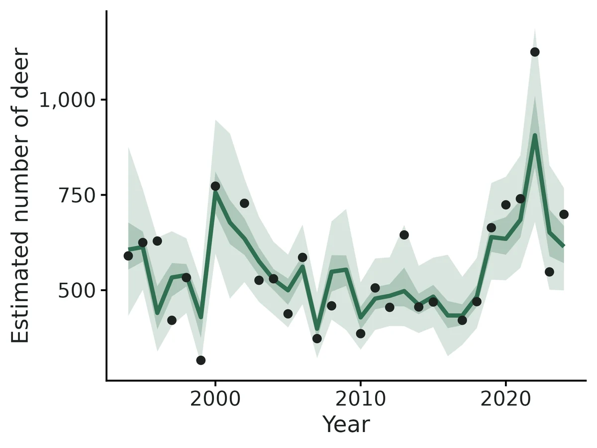
What this means
- The estimated true population changed by +0.1% per year on average between 1994 and 2024 (95% credible interval -1.4% to +1.3%).
- Estimated true abundance (on the scale of the animals counted) in 2024: 614 (95% credible interval 499 to 768). If counts miss a constant fraction of animals this is an index of abundance, not a census.
- Equilibrium abundance (where growth averages zero, at average covariates): 536 (95% credible interval 478 to 599).
- An increase of one standard deviation (20) in Mean winter snow depth (cm) is associated with a -15.3% change in the annual growth multiplier (95% credible interval -22.2% to -7.0%; P(effect > 0) = 0.00). At average abundance the population is expected to change by +19.9% in a year with snow depth at its 10th percentile (30.9 cm) vs -16.4% at its 90th percentile (74.5 cm). This is an association, not proof that snow depth causes the change.
- Counting error (observation SD 0.18, 95% CI 0.03-0.28) is estimated to be larger than real year-to-year variation (process SD 0.10, 0.00-0.26), so single year-to-year changes in raw counts should not be read as real population changes.
- Because the prior allows only b between -2 and 0, the credible interval for b can never include 0, so it is not evidence that density dependence exists; b from a single count series is overestimated (here -0.59 vs true -0.30).
- Posterior predictive check: the variability (Bayesian p = 0.61) and lag-1 autocorrelation (p = 0.75) of year-to-year changes match the observed counts, so there is no sign of misfit.
- Formal test for density dependence (Gompertz parametric-bootstrap likelihood ratio, 199 simulated series): p = 0.585; the counts are consistent with density-independent growth, but this test has little power.
More figures
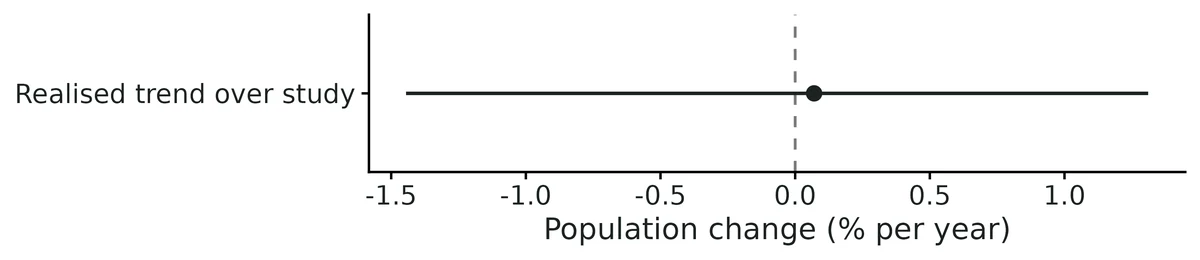
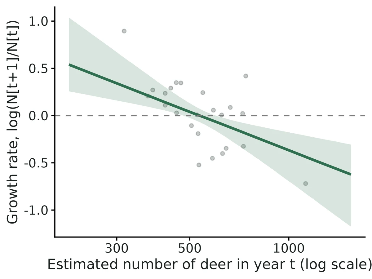
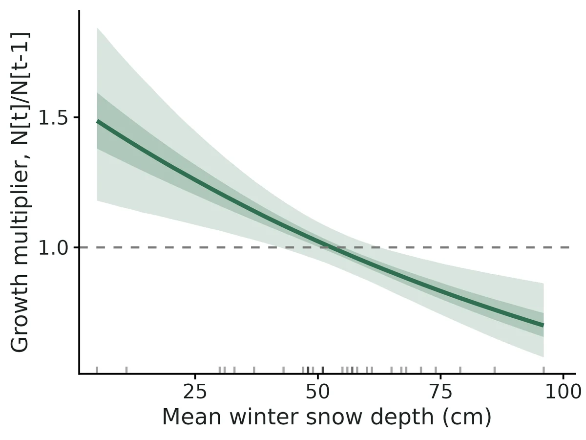
Figures are the module's default publication figures, reduced for the web. The report also saves them as PDF and full-resolution PNG.
Planted truth at the example's design
Before trusting the example's results, the module was run on many simulated data sets with the same design and known true values. Each row is one quantity: did the method get it back? (What the thresholds are.)
What OPEN means here. The module works (it passes at its default design), but at this example's design not every quantity passed the planted-truth check, so CascadiaTools does not certify those. 5 of the 8 quantities checked passed outright. For density dependence b, sd process, sd observation, the estimate was biased (by up to 59%); don't interpret those at this design. The quantities that passed can be used as reported. With your own data, the report would say the same and suggest what would help: more data, a simpler model or a different estimator. More on DONE and OPEN.
Why, for this example:
Estimand-specific. Trend, N_final, equilibrium_N and the snow effect pass planted truth (bias <= 4.2%, coverage 0.94-0.97), convergence (R-hat <= 1.006, ESS >= 684) and the PPC, and can be reported. Density dependence b (-59% bias), process SD (+23%) and observation SD (-13%) fail planted truth at this design, so the researcher's density-dependence question is not answered.
| This example | one herd counted over 31 winters (28 counted, 3 missed), Bayesian Gompertz model with a snow covariate |
|---|---|
| Design the module was validated at | one 25-year count series, Bayesian state-space model with density dependence and one covariate on growth |
The example series is a little longer (31 years, 28 counted) than the 25-year validated Bayesian design. At that design the covariate effect (-2.2% bias, coverage 0.958), final abundance (+2.7%) and equilibrium abundance (+0.9%) passed. Density dependence b (-62%), process SD (+31%) and observation SD (-15%) failed. Even at 50 years b was still 30% too strong, so the example's density-dependence estimate cannot be trusted.
These calls sit close to the pass/fail line. With another 93 simulated data sets they could come out the other way, so read them as “about at the limit” rather than as a clear pass or fail.
- density_dependence_b (✗ FAIL): coverage 0.892 against a minimum of 0.882.
5 of 8 rows pass; 1 is borderline.
| Quantity | True value | Average estimate | Bias | Allowed bias | Coverage (needed) | Result |
|---|---|---|---|---|---|---|
| growth_beta_snow_depth_cm | -0.15 | -0.156 | -4.2% | ±10.0% | 0.97 (0.882) | ✓ PASS |
| growth_effect_pct_snow_depth_cm | -13.9 | -14.4 | -3.5% | ±10.0% | 0.97 (0.882) | ✓ PASS |
| N_final | 517.3 | 526.9 | +1.9% | ±10.0% | 0.96 (0.882) | ✓ PASS |
| equilibrium_N | 500 | 503.8 | +0.8% | ±10.0% | 0.96 (0.882) | ✓ PASS |
| realised_trend_pct_per_year | 0.118 | 0.121 | +3.2% | ±170.7%† | 0.94 (0.882) | ✓ PASS |
| density_dependence_b | -0.3 | -0.476 | -58.6% | ±16.5%† | 0.89 (0.882) | ✗ FAIL ≈ borderline |
| sd_process | 0.1 | 0.123 | +23.1% | ±12.6%† | 0.98 (0.882) | ✗ FAIL |
| sd_observation | 0.15 | 0.13 | -13.4% | ±10.0% | 0.99 (0.882) | ✗ FAIL |
Limits that matter
- Density dependence is not recoverable from a single count series (Knape 2008): b biased -59% at this design; in bayes the U(-2,0) prior means its interval never contains 0.
- Process and observation SDs are biased (+23% and -13% here); trend and abundance intervals remain valid.
- Constant detection is assumed: herd size is an index on the count scale, and a change in sightability would look like a trend.
- 'No clear trend' is weak evidence: a single series declining 5%/yr is detected with power 0.29 after 20 years and 0.49 after 30.
- Bayes density-dependence fits can mix slowly: 7% of fast-setting replicates missed the convergence rule; the real fit (4 x 40,000) had min ESS 684.
- Covariate effects are associations, not causes.
- The Gompertz bootstrap test of density dependence holds its false-positive rate but has 2-6% power at b = -0.3.
All known limits from the module's validation record
- Variance components from one series. sd_process is biased (REML -17% at 25 yr; Bayes +31%) and sd_observation is biased in the Gompertz and Bayes models. Trend and abundance intervals stay valid. Pooling sites (
marss) or an independent estimate of counting error (prior_sd_observation) fixes it. Density dependence is not recoverable from a single count series (Knape 2008; Auger-Methe et al. 2016). Point estimates of b are overestimated by 30-140% depending on length and engine. The profile interval for b excludes 0 in 47% of series without density dependence.
- The bootstrap LRT holds its size (0.04-0.07) but has almost no power at 15 years.
- In
bayesthe U(-2, 0) prior means the interval for b never contains 0. - The interpretation text states all of this.
- equilibrium_N (Gompertz ML) is undefined when b is near 0. The mean of the MLEs is dominated by huge values and coverage is 0.889 at 30 yr. The report suppresses K when its interval spans more than a 20-fold range.
- Trend intervals are conservative. The false-positive rate is 0.025, and coverage is 0.97-1.0 below 20 years. Power is therefore lower than with plug-in intervals, which are invalid (coverage 0.81).
process_cov: equalvarcov(MARSS EM) converged in only 75% of replicates. Treat process_corr as exploratory.loglinearwith 3 sites x 10 years: 14.5% of fits have a singular Hessian. It also does not separate process from observation error.- Constant detection is assumed. Abundance is on the count scale, and a trend in detectability is indistinguishable from a population trend.
- The importance sampler for ML abundance intervals can have low ESS (<200) for Gompertz fits with a strongly curved likelihood. The fit then adds a note.
- Bayes DD fits mix slowly when b is poorly identified. In the 60-year cross-check, minimum ESS was 188 at 4 x 40,000 iterations; the report flags runs below ESS 400.
- REML trend intervals are very conservative when counting error dominates. At 20 years with sd_process 0.06 and sd_observation 0.25, a +4%/yr trend was never detected (power 0.000, false-positive rate 0.000, coverage 1.000), whereas GLS with the true variances would detect it in 60% of series. The intervals are valid but can be about 3x wider than necessary; see "Independent verification". The report now says that "no clear trend" is not evidence of stability and points to a power analysis.
loglineartrend intervals are too narrow when the population itself wanders (random walk with drift plus counting error): coverage 0.825 at 4 sites x 25 years. The report warns when the fitted AR(1) correlation exceeds 0.9 and always says to compare withmarss/exponential.
How this module was validated
- 100-200 simulated datasets per design across five engines: single-series REML trend, multi-site MARSS, Gompertz maximum likelihood, log-linear GLMM and Bayesian state-space. The Bayesian fits used 3 chains x 12,000 iterations, 4,000 burn-in. To pass, bias had to be within 10% (or 3 Monte Carlo SE) and coverage (how often the 95% interval contained the truth) at least 0.885-0.904.
- Passed: trends, final abundance, covariate effects on growth and equilibrium abundance. Failed: density dependence at the default noise levels (Gompertz ML -96% at 30 years, Bayes -62% at 25 years) and process SD from a single series (REML -17%).
- Harder designs: 12-year series, 30% missing years and multi-site series with gaps all kept trend coverage. The log-linear model with 3 sites x 10 years failed on convergence (85.5% converged).
- Negative control: ignoring counting error made density dependence look 2.6 times stronger (coverage 0.275) and dropped final-abundance coverage to 0.000.
- False-positive rates: 0.025 for the REML trend, 0.045 for MARSS and 0.031 for the Bayesian covariate. The Gompertz profile interval for b excluded 0 in 47% of series with no density dependence, so the bootstrap test (0.04-0.07) is used instead.
- Cross-checks: the module matched the MARSS package (log-likelihood within 6e-4) and MASS glm.nb (within 1e-6), and the Bayesian fits agreed with Kalman maximum likelihood on long series.
- Power: a 5%-per-year decline in one population reached 0.71 power only at 40 years, while 4 sites over 25 years gave 0.735 for a 3% decline. A separate verifier agent found that b can be recovered (Gompertz ML at 40 years, b = -0.5, process noise larger than counting error), but the Bayesian model still overstated it by 33%.
Every run uses the acceptance gate described on the validation page. The full record follows, section by section, exactly as kept in the module's VALIDATION.md.
Settings and pass/fail rule used for every run
Every number below was produced by the scripts named next to it. Rerun the full recovery set with bash dev/timeseries/run_recover.sh <nsim> <cfg...> (configs in dev/timeseries/<cfg>.yaml, results in results/timeseries/recover_<cfg>/). bin/Rscript dev/timeseries/gate_md.R regenerates the tables in the appendix. All recoveries used the module's fast_settings:
- Bayes: 3 chains x 12,000 iterations, 4,000 burn-in, thin 4; the long design used 30,000 / 10,000 / 10.
- ML/REML: 300 trajectory draws, no bootstrap density-dependence test inside each replicate.
The gate is recovery_gate() with its fixed thresholds:
bias <= max(10% of truth, 3 MC SE); - coverage >= 0.95 - 3 MC SE (0.885 at n = 100, 0.904 at n = 200);
- >= 90% of replicates converged.
Default parameters (module$defaults): growth_rate_mu = -0.03 (-2.96%/yr), sd_process = 0.10, sd_observation = 0.15, density_dependence_b = -0.3, equilibrium_N = 500, growth_beta = -0.15 per SD, start N = 500. Final run: 2026-10-20, after the SIR change to ML abundance intervals (below).
Verdict: OPEN (estimand-specific)
| What a researcher would report | Status | Evidence (default design unless stated) |
|---|---|---|
Trend (% per year), single series, exponential (REML) | PASS | 25 yr: bias -5.9%, coverage 0.975; 12 yr and 30% missing years also pass |
Trend, several sites, marss (pooled REML) | PASS | 4 sites x 25 yr: bias -4.6%, coverage 0.955; 2 sites x 15 yr with gaps passes; separate per-site trends pass |
Trend, loglinear (glmmTMB, NB + AR(1)) | PASS at 5 sites x 20 yr | 3 sites x 10 yr fails convergence (85.5% converged) |
True abundance in the last year (N_final) | PASS | exponential 0.945, gompertz 0.920, bayes 0.938 coverage; bias < 3% |
Covariate effect on growth (bayes) | PASS | bias -2.2%, coverage 0.958; false-positive rate 0.031 with effect = 0 |
Equilibrium abundance (bayes) | PASS | bias +0.9%, coverage 0.969 |
| Observation SD | PASS only for exponential at >= 25 yr, marss, and bayes with an informative prior | single-series Gompertz -40%; Bayes -15% |
| Process SD | FAIL for a single series | REML -17% at 25 yr (-24% at 12 yr); Bayes +31%; passes only for marss (pooled over sites) and Bayes with an observation-error prior |
Density dependence b | FAIL at the default noise ratio (sd_o > sd_p) | Gompertz ML -96% at 30 yr, -49% at 60 yr; Bayes -62% at 25 yr, -30% at 50 yr. This is the Knape (2008) problem; see below. Independent check: with b = -0.5 and sd_p > sd_o, Gompertz ML at 40 yr was unbiased (coverage 0.96), Bayes still -33% |
Bottom line for researchers:
- Trends, the trajectory of true abundance and covariate effects on growth are recovered with honest intervals at realistic designs.
- Process and observation SDs from one series of 25 years are biased by about 15-40%. Do not over-interpret them.
- Density dependence from one count series is not recoverable without independent information on counting error. Even with it, b is overestimated (bayes_obsprior: -52%).
1. Recovery at the default design and harder designs
Single series (exponential growth with drift, REML):
| design | trend bias | trend coverage | N_final coverage | sd_obs bias | sd_proc bias | gate |
|---|---|---|---|---|---|---|
| 25 yr (default, nsim 200) | -5.9% | 0.975 | 0.945 | -2.4% | -16.9% | trend, N, sd_obs PASS; sd_proc FAIL |
| 12 yr (hard) | -7.4% | 0.985 | 0.955 | -16.2% | -23.7% | trend, N PASS; SDs FAIL |
| 25 yr, 30% of years missing | -5.6% | 0.990 | 0.930 | -8.0% | -20.7% | as default |
25 yr, estimation: ml (comparison) | -5.9% | 0.675 | 0.960 | +6.9% (cov 0.84) | -59.8% (cov 0.575) | trend FAIL |
Why REML is the default:
- Plain ML estimates sd_process at exactly 0 in many series, and the trend interval then collapses (coverage 0.675).
- REML integrates the variances out on a grid (flat prior on both SDs), which keeps trend intervals honest.
- The price is conservatism: coverage is 0.97-1.0 below 20 years, and the false-positive rate is 0.025 instead of 0.05 (section 4).
dev/timeseries/prior_study.R(results/timeseries/prior_study.csv) compared four ways of handling the variances at 25 years (sd_p 0.1, sd_o 0.15). Each pair is coverage / power:- plug-in GLS: 0.81 / 0.42 (invalid);
- log-uniform prior: 0.91 / 0.28;
- sqrt prior: 0.95 / 0.20;
- flat prior: 0.968 / 0.165.
- Flat was kept because it is the only option with coverage >= 0.90 in every scenario studied.
sd_process (single series) is the one default-design estimand that fails:
- REML puts it on the boundary (0) in about 14% of 25-year series.
dev/timeseries/sd_estimator_study.Rtried the grid-posterior median (+12%) and mean (+20%). No point estimator came within 10% at 25 years. At 50 years REML bias is -6.6%.- Interval coverage is fine (0.98). The point estimate is not reliable, and the interpretation text says so when it is at the boundary.
Multi-site (marss, pooled REML, shared trend), nsim 200:
| design | trend bias | trend coverage | sd_obs | sd_proc | gate |
|---|---|---|---|---|---|
| 4 sites x 25 yr (default) | -4.6% | 0.955 | +0.6% / 0.980 | -4.1% / 0.925 | all PASS |
| 2 sites x 15 yr, 20% missing (hard) | -3.1% | 0.980 | -5.3% / 0.950 | -12.2% / 0.965 | all PASS (sd_proc within 3 MC SE) |
| 4 sites, separate trends (-5, -3, 0, +2%/yr) | -3 to -4% | 0.945-0.960 | PASS | PASS | all PASS |
estimation: ml (MARSS, Hessian CIs) | -2.6% | 0.877 | PASS | -16.5% / 0.791 | FAIL (cov) |
process_cov: equalvarcov (MARSS EM, process_corr 0.5) | -6.8% | 0.920 | +2.0% | -12.7% | FAIL: only 150/200 converged; process_corr +14.8% |
Density dependence, single series (gompertz, exact Kalman ML), nsim 200:
| design | b (true -0.3) | equilibrium_N | N_final coverage | sd_obs | sd_proc |
|---|---|---|---|---|---|
| 30 yr (default for this model) | mean -0.589 (-96%), cov 0.915 | cov 0.889; mean of MLEs 3.4e7 (heavy tail when b ~ 0) | 0.920 PASS | -40% | +7.3% PASS |
| 15 yr | -0.710, cov 0.875 | cov 0.765 | 0.895 FAIL | -44% | -18% |
| 60 yr | -0.447 (-49%), cov 0.915 | cov 0.930* | 0.910 PASS | -30% | +13% |
\* equilibrium_N passes the gate at 60 years only formally: the mean of the MLEs is dominated by a few series with b near 0, which makes 3 MC SE enormous. Report K only when its interval spans less than a 20-fold range. The interpretation enforces that rule.
Fix made in this round (ML abundance intervals). Abundance intervals for the ML engines previously drew parameters from the asymptotic normal (Hessian) distribution. That collapsed to zero width whenever sd_observation was estimated at 0, and exploded when b was drawn near -2. The coverage of Gompertz N_final was 0.573. They now use adaptive sampling-importance- resampling from the likelihood (kalman.R kf_sir):
- flat priors, with the SDs flat on the SD scale;
- a multivariate-t proposal, re-centred over 3 pilot rounds;
- typical importance ESS of 1,300-4,400 for exponential and 200-1,300 for Gompertz, out of 20,000 proposals; the fit notes when ESS < 200.
After the change, N_final coverage is 0.920 (Gompertz, 30 yr) and 0.960 (exponential ML, previously 0.79).
Bayesian state-space model (bayes, Nimble), nsim 100, 24 s per replicate:
| design | covariate effect (true -13.9%/SD) | N_final | equilibrium_N | b (true -0.3) | sd_obs | sd_proc | realised trend |
|---|---|---|---|---|---|---|---|
| 25 yr, DD + covariate (default) | -1.6%, cov 0.958, power 0.938 | +2.7%, 0.938 | +0.9%, 0.969 | -0.486 (-62%) | -15% | +31% | abs bias +0.22 %/yr (truth ~0), cov 0.938: FAIL |
| 15 yr | +2.2%, 0.960, power 0.606 | PASS | PASS | -0.631, cov 0.869 | -6% | +38% | PASS |
| 50 yr | -0.1%, 0.990, power 1.0 | PASS | PASS | -0.389 (-30%) | -8% PASS | +23% | PASS |
| 25 yr, 20% years missing | -1.2%, 0.960, power 0.84 | PASS | PASS | -70% | -13% | +34% | FAIL (as default) |
25 yr, no DD (density_dependence: false) | +3.8%, 0.970 | PASS | n/a | n/a | -11% | +17% | PASS (r0 +3.1%, cov 0.99) |
| 25 yr + informative prior sd_obs ~ N+(0.15, 0.03) | -2.9%, 0.970 | PASS | PASS | -0.457 (-52%) | -2.3% PASS | +11.5% PASS | PASS |
- Convergence (R-hat < 1.05 for every reported quantity) held in 96-100% of replicates.
- The SD biases come from a half-normal(0, 1) prior meeting the Knape/Dennis trade-off. With an informative observation-error prior (Knape's recommended cure) everything except b passes.
- The realised trend fails only at the DD default design. There the true realised trend is about 0 (a population at equilibrium), so the 10% relative tolerance is meaningless. Its absolute bias is 0.2 percentage points per year against an interval width of 2.8.
Log-linear GLMM (loglinear), nsim 200:
- 5 sites x 20 yr: trend bias -0.1%, coverage 0.938, power 0.933; covariate +1.6%, coverage 0.943. All PASS.
- 3 sites x 10 yr: estimates fine (coverage 0.92-0.94), but only 171/200 fits converged (glmmTMB pdHess false: the AR(1) variance collapses). FAIL (conv).
2. Negative controls (the gate can fail)
Ignoring observation error (observation_error: false, the classic diffusion/AR(1) regression on log counts):
| model | estimand | with observation error | ignoring it |
|---|---|---|---|
| Gompertz, 30 yr, true b = -0.3 | density_dependence_b | -0.589 (cov 0.915) | -0.786 (-162%, cov 0.275) |
| Gompertz | sd_process | +7%, cov 0.930 | +82.5%, cov 0.005 |
| Gompertz | N_final coverage | 0.920 | 0.000 (counts treated as truth) |
| Exponential, 25 yr | sd_process | -17%, cov 0.980 | +133%, cov 0.000 |
| Exponential | N_final coverage | 0.945 | 0.000 |
Ignoring counting error makes density dependence look 2.6x stronger than the truth. This is the regression-to-the-mean artefact of Shenk et al. (1998), Dennis et al. (2006) and Knape (2008). Other controls that fail as they should:
- plain ML instead of REML (trend coverage 0.675);
- MARSS ML (trend coverage 0.877).
3. False-positive rates with effect = 0
| model, design | quantity | rejection rate (nominal 0.05) |
|---|---|---|
| exponential, 25 yr, mu = 0 (nsim 200) | trend interval excludes 0 | 0.025 (conservative) |
| marss, 4 x 25, mu = 0 (nsim 200) | trend | 0.045 |
| loglinear, 5 x 20 (nsim 200) | trend / covariate | 0.077 / 0.071 (MC SE 0.019) |
| bayes, 25 yr, growth_beta = 0 (nsim 100) | covariate effect on growth | 0.031 |
| gompertz, 30 yr, b = 0 (nsim 200) | profile interval for b excludes 0 | 0.472: not a valid test |
| gompertz, bootstrap LRT (199 or 99 simulations), b = 0 | p < 0.05 | 15 yr: 0.070 (MC SE 0.026); 30 yr: 0.040 (MC SE 0.020) |
| gompertz, bootstrap LRT, b = -0.3 (power) | p < 0.05 | 15 yr: 0.060 (MC SE 0.024); 30 yr: 0.020 (MC SE 0.014) |
Source: dev/timeseries/ddtest_study.R (logs/timeseries_ddtest.log, logs/timeseries_ddtest30.log).
How to use these results:
- Test density dependence with the bootstrap LRT, never with the interval for b.
- With realistic noise (sd_p 0.1, sd_o 0.15) the test has essentially no power at 15 or even 30 years (rejection rate at b = -0.3 is no higher than at b = 0), as Knape (2008) predicts. A non-significant test therefore says nothing about whether density dependence is absent.
4. Power: years of monitoring to detect a decline
core/run.R power with dev/timeseries/power_exp5.yaml: single series, exponential REML, -5%/yr (growth_rate_mu = -0.0513), sd_process 0.1, sd_observation 0.15, nsim 200 per point. Results are in results/timeseries/power_5pct/. Power = share of 95% trend intervals excluding 0.
| years | 8 | 10 | 12 | 15 | 20 | 25 | 30 | 40 |
|---|---|---|---|---|---|---|---|---|
| power | 0.025 | 0.040 | 0.045 | 0.115 | 0.290 | 0.400 | 0.485 | 0.710 |
| trend coverage | 0.995 | 0.995 | 0.995 | 1.000 | 0.980 | 0.970 | 0.980 | 0.945 |
Decline size at 20 years (dev/timeseries/power_exp20.yaml, vary growth_rate_mu, nsim 200):
| decline %/yr | 0 | 1 | 2 | 3 | 5 | 7 | 10 |
|---|---|---|---|---|---|---|---|
| power | 0.015 | 0.040 | 0.045 | 0.095 | 0.260 | 0.485 | 0.840 |
What this means for managers:
- With real year-to-year variation of 10% (sd_process 0.1), a single monitored population declining 5% a year is detected with 80% power only after more than 40 years.
- The drift of a random walk is inherently hard to estimate, and the module's integrated intervals are deliberately conservative.
- Monitoring several sub-populations with a shared trend helps a lot:
marssat 4 sites x 25 years has power 0.735 for a 3%/yr decline, against 0.145 for one site. - Plan with
--vary n_sitesas well asn_years.
5. Cross-checks against independent implementations
Source: dev/timeseries/crosscheck.R, logs/timeseries_crosscheck3.log.
| engine | independent route | agreement |
|---|---|---|
| EGSS Kalman ML (3 datasets, 30 yr) | MARSS package (B = 1, x0 at t = 0) | log-lik within 6e-4; mu within 8e-7; SDs within 2.3e-5 |
| EGSS REML (3 datasets with gaps) | brute-force numerical integration of the differenced-data likelihood over mu, maximised | SDs within 3.4e-4 (the larger difference is at the sd = 0 boundary) |
| GSS (Gompertz) Kalman ML (3 datasets, 40 yr) | MARSS with B estimated | identical log-lik and estimates (<= 1e-5) when MARSS is started at the module MLE. From MARSS's default start, 2 of 3 fits stopped at a lower likelihood near b = 0 (11.76 vs 12.29; 11.11 vs 12.02); the module's multi-start optimiser found the higher maximum |
| multi-site ML (3 datasets) | hand-written multivariate Kalman filter + optim | log-lik identical; parameters within 5e-6 |
| pooled multi-site REML (shared and separate trends) | brute-force integration over the trend(s) | SDs within 3e-7 |
| pooled REML with 1 site | single-series REML | identical to 1e-12 (estimates and intervals) |
| bootstrap LRT statistic | 2 x (MARSS GSS - MARSS EGSS log-lik) | within 0.002 |
| loglinear (glmmTMB, ar1 = FALSE, 1 site) | MASS::glm.nb | coefficients within 1e-6; SEs within 5e-4 |
| Bayes (Nimble), exponential, 60 yr | Kalman ML | mu -0.0043 vs -0.0044; N_final 386 vs 385; SDs within 0.015 |
| Bayes, Gompertz, 60 yr | Kalman ML | N_final 574 vs 567; b -0.735 vs -0.230 (the Knape non-identifiability: the two routes settle on different splits of the noise) |
6. Example data
example/herd_counts.csv (31 winters, 3 not flown) was simulated with dev/timeseries/make_example.R. The true values are b = -0.3, K = 500, sd_p 0.10, sd_o 0.15, N_final 643 and a snow effect of -13.9%/SD.
The bayes fit (example/config.yaml) gives:
- N_final 614 (95% CrI 499-768);
- K 536 (478-599);
- snow effect -15.3% (-22.2 to -7.0);
- sd_p 0.10 and sd_o 0.18.
All of these cover the truth. b = -0.59 (-1.11 to -0.29) misses the true -0.3, which is the documented overestimation of density dependence.
The gompertz fit's bootstrap LRT gives p = 0.585, i.e. no detectable density dependence from this one series.
Independent verification (2026-10-20, separate agent)
Everything below was produced by a verifier that did not build the module. Scripts: dev/timeseries/verify/. Results: results/timeseries/verify/<scenario>/ and results/timeseries/verify_rerun_<cfg>/. Logs: logs/timeseries_verify_*.log.
Literature and code check
- GSS/EGSS equations match Dennis et al. (2006) as restated by Dennis & Ponciano (2014): X_t = a + c X_{t-1} + E_t, Y_t = X_t + F_t. The module's c = 1 + b and a = -b log K give the stationary mean log K (= a/(1 - c)). EGSS is c = 1. Unlike Dennis et al. (2006), which start from the stationary distribution, the module estimates the initial state freely (the nonstationary variant; MARSS x0 at t = 0). It is stated in the methods text.
- REML for EGSS: the differenced log counts have mean mu k_i, variance k_i sd_p^2 + 2 sd_o^2 and lag-1 covariance -sd_o^2 (Staples et al. 2004; Humbert et al. 2009). Code (
egss_S,egss_negreml) matches. - Bayes: equilibrium log K = xbar - r0/b follows from setting the expected change r0 + b(x - xbar) to 0. Priors in code match README/methods.
- Knape (2008): b is weakly identified when both variances are unknown, and how badly depends on the parameter values; a known observation variance removes the problem. This matches the module's text and the new parameter-dependence result below.
- Fixed: the exponential (REML) methods text claimed a GLS trend with a t-based interval. The code reports the mean and quantiles of the grid-integrated mixture. The methods text and the
reml.Rheader now describe what the code does. - The simulators share no code with fit() beyond
ts_drop_years, and the independent simulators below share none at all.
Rerun of the builder's recoveries (same configs, nsim as stated)
exp_default (200), marss_default (200), gomp_null (200), bayes_default (100) and exp_noobs (200) reproduced the appendix tables exactly. For example: exp_default trend bias -5.89%, coverage 0.975; marss_default trend coverage 0.955, power 0.735; gomp_null interval for b excludes 0 in 0.472; bayes_default covariate coverage 0.958 and b -62%; exp_noobs sd_process +133% and N_final coverage 0.
Independent planted truth (own simulators, indep_recovery.R; module fit() with fast_settings; core summarise_recovery + recovery_gate)
| scenario (design differs from builder's) | estimand | truth | rel. bias | coverage | power / FPR | gate |
|---|---|---|---|---|---|---|
| exp_v: 20 yr, mu +0.04, sd_p 0.06, sd_o 0.25, 15% missing, nsim 200 | trend | +4.08%/yr | -2.4% | 1.000 | power 0.000 | PASS (see limit 10) |
| N_final | 317 | +0.9% | 0.965 | PASS | ||
| sd_observation | 0.25 | -10.4% | 0.945 | FAIL (bias, just over 10%) | ||
| sd_process | 0.06 | +14.1% | 0.970 | PASS (within 3 MC SE) | ||
| exp_v_null (mu = 0) | trend | 0 | 1.000 | FPR 0.000 | PASS | |
exp_v_ml (estimation: ml, negative control) | trend | -3.7% | 0.825 | 0.74 | FAIL, as expected | |
exp_v_noobs (observation_error: false, negative control) | sd_process / N_final | +453% / | 0.000 / 0.000 | FAIL, as expected | ||
| marss_v: 6 sites x 18 yr, mu -0.05, sd_p 0.08, sd_o 0.20, 10% missing | trend / sd_obs / sd_proc | -1.3% / +0.2% / -6.3% | 0.935 / 0.980 / 0.965 | power 0.995 | all PASS | |
| marss_v_null (mu = 0) | trend | 0 | 0.935 | FPR 0.065 (MC SE 0.017) | PASS | |
| ll_v: 8 sites x 15 yr, NB size 5, AR(1) rho 0.3, mu +0.02, covariate -0.2/SD | trend / covariate | +1.4% / +0.5% | 0.926 / 0.952 | 0.37 / 0.98 | PASS (189/200 converged) | |
| ll_v_null (both effects 0) | trend / covariate | 0 | 0.941 / 0.941 | FPR 0.059 / 0.059 | PASS | |
ll_rw: random walk + counting error (4 x 25), fitted by loglinear | trend | -2.96%/yr | -1.2% | 0.825 | FAIL (limit 11) | |
| gomp_v: 40 yr, b -0.5, K 2000, sd_p 0.15, sd_o 0.10, nsim 200 | b | -0.5 | -0.01% | 0.960 | PASS | |
| equilibrium_N | 2000 | median -0.8% (mean dominated by tail) | 0.940 | PASS | ||
| N_final / sd_proc | +0.9% / -9.6% | 0.935 / 0.960 | PASS | |||
| sd_observation | 0.10 | -36% | 0.955 | FAIL (bias) | ||
| gomp_v_noobs (negative control) | b / sd_proc / N_final | -32% / +19% / | 0.865 / 0.625 / 0.000 | FAIL, as expected | ||
| bayes_v: 30 yr, b -0.5, K 1200, sd_p 0.12, sd_o 0.10, 10% missing, rain (+0.10/SD) and temperature (0) on growth, nsim 100 (97 converged) | rain effect | +10.5%/SD | +0.3% | 0.969 | power 0.76 | PASS |
| temperature effect (null) | 0 | 0.918 | FPR 0.082 (MC SE 0.028) | PASS | ||
| N_final / K | +0.8% / +0.5% | 0.938 / 0.928 | PASS | |||
| sd_obs / sd_proc | +5.8% / -3.0% | 1.000 / 1.000 | PASS | |||
| b | -0.5 | -33% | 0.918 | FAIL (bias) |
What this adds to the builder's results:
- Trends, abundance, equilibrium N and covariate effects pass at independent designs too. False-positive rates are 0.059-0.082, except REML single-series trends, which are conservative (0.000 here, 0.025 at the default).
- Density dependence is parameter-dependent, not uniformly unrecoverable. With b = -0.5 and process noise larger than counting error, 40 years of Gompertz ML recovered b without bias (coverage 0.96). The Bayes model (U(-2, 0) prior, 30 yr) still overstated it by 33%. The builder's FAIL for b holds at its own noise ratio (sd_o > sd_p) and should not be read as "never". Without independent evidence about the noise ratio, a researcher cannot tell which regime applies, so the report's caution stays.
- Power of REML single-series trends (limit 10). Oracle comparison (
oracle_trend.R, 1000 series at the exp_v design): GLS with the true variances had coverage 0.936, power 0.595 and interval width 0.070 (log scale). Plug-in REML GLS had coverage 0.856 (invalid) and power 0.58. The module had coverage 1.000, power 0.000 and width 0.196. Validity is kept at a high price. The builder's prior study found the same trade-off at the default design. This is a design limit to report, not a bug. loglinearunder random-walk dynamics (ll_rw_rho.R): the fitted AR(1) rho exceeded 0.9 in 66% of series (median 0.945). Coverage was 0.89 for those and 0.69 for the rest, so the rho warning catches only some cases. The fixed caveat sentence therefore states the 0.825 coverage for everyloglinearfit.
Usability (as a non-coding user would meet it)
fitonexample/config.yamlreproduced the reported example: N_final 614 (499-768), K 536 (478-599), snow effect -15.3% (-22.2 to -7.0), b -0.59. Max R-hat 1.006, min ESS 684, PPC p = 0.61 / 0.75. Every number in the interpretation was checked by hand against the estimates (half-life log 0.5 / log(1 - 0.591) = 0.78 yr; compounding of trends; 10th/90th percentile growth).Messy data (
dev/timeseries/verify/messy/):- wrong column name: clear message listing the columns present;
- "n/a" in counts: clear message;
- duplicated year: clear message;
- covariates with a model that cannot use them: clear message;
- misspelled site name ("Nrth Fork" in 2 of 25 years): previously passed check_data silently (MARSS would have fitted a fifth site or stopped with an unhelpful error).
- Figures: trend, variances, trace, coefficients, growth_snow_depth_cm and the MARSS residual panels were opened. No overlaps or clipping, and units are correct. The growth curve crosses 1 at about 53 cm, matching r0 ~ 0 at the covariate mean. Gompertz has no
trendfigure because it has no trend estimand.
Changes made by the verifier (text, checks and interpretation only; no change to simulate() or fit() numerics)
R/common.Rts_check_data: flags site names that differ only in case/punctuation, or by at most 2 edits when one has fewer than half the other's counted years, plus any site with fewer than 3 counted years. Non-numeric-value messages now give the spreadsheet line as well as the data row.module.Rmethods text (exponential REML) andR/reml.Rheader: describe the integrated-mixture trend interval actually computed.module.Rinterpretation:- the half-life sentence is given only when the interval for b excludes 0, and is flagged as likely too short;
- when the Gompertz profile interval for b reaches the -2 search limit, the report says so;
- the advice to use
prior_sd_observationnow says it needsmodel: bayes(the Gompertz ML fit ignored it); - "no clear trend" now adds the compounded range and a pointer to power analysis;
loglinearwarns when AR(1) rho > 0.9 and states the 0.825 random-walk coverage.
- Example reports regenerated with these texts (
results/timeseries/example*/). No gate threshold was changed. Nothing incore/was changed.
Appendix: all recovery tables
bayes_default (nsim 100, 0 crashed, 24.0 s/rep; config dev/timeseries/bayes_default.yaml)
| estimand | truth | mean est | rel. bias | coverage | CI width | power | converged | gate |
|---|---|---|---|---|---|---|---|---|
| density_dependence_b | -0.3 | -0.486 | -62.0% | 0.917 | 0.762 | 96/100 | FAIL (bias) | |
| equilibrium_N | 500 | 505 | +0.9% | 0.969 | 260 | 96/100 | PASS | |
| growth_beta_winter_severity | -0.15 | -0.153 | -2.2% | 0.958 | 0.177 | 0.938 | 96/100 | PASS |
| growth_effect_pct_winter_severity | -13.9 | -14.2 | -1.6% | 0.958 | 15.3 | 96/100 | PASS | |
| N_final | 513 | 524 | +2.7% | 0.938 | 212 | 96/100 | PASS | |
| realised_trend_pct_per_year | -0.0522 | 0.164 | +116.3% | 0.938 | 2.81 | 96/100 | FAIL (bias) | |
| sd_observation | 0.15 | 0.128 | -14.8% | 0.990 | 0.225 | 96/100 | FAIL (bias) | |
| sd_process | 0.1 | 0.131 | +30.6% | 1.000 | 0.233 | 96/100 | FAIL (bias) |
bayes_hard (nsim 100, 0 crashed, 22.1 s/rep; config dev/timeseries/bayes_hard.yaml)
| estimand | truth | mean est | rel. bias | coverage | CI width | power | converged | gate |
|---|---|---|---|---|---|---|---|---|
| density_dependence_b | -0.3 | -0.631 | -110.2% | 0.869 | 1.19 | 99/100 | FAIL (bias cov) | |
| equilibrium_N | 500 | 499 | -0.3% | 0.960 | 730 | 99/100 | PASS | |
| growth_beta_winter_severity | -0.15 | -0.148 | +1.1% | 0.960 | 0.267 | 0.606 | 99/100 | PASS |
| growth_effect_pct_winter_severity | -13.9 | -13.6 | +2.2% | 0.960 | 23.2 | 99/100 | PASS | |
| N_final | 512 | 518 | +1.6% | 0.990 | 247 | 99/100 | PASS | |
| realised_trend_pct_per_year | 0.0599 | 0.25 | -45.4% | 0.980 | 5.74 | 99/100 | PASS | |
| sd_observation | 0.15 | 0.141 | -6.3% | 1.000 | 0.288 | 99/100 | PASS | |
| sd_process | 0.1 | 0.137 | +37.5% | 1.000 | 0.3 | 99/100 | FAIL (bias) |
bayes_long (nsim 100, 0 crashed, 50.0 s/rep; config dev/timeseries/bayes_long.yaml)
| estimand | truth | mean est | rel. bias | coverage | CI width | power | converged | gate |
|---|---|---|---|---|---|---|---|---|
| density_dependence_b | -0.3 | -0.389 | -29.7% | 0.930 | 0.465 | 100/100 | FAIL (bias) | |
| equilibrium_N | 500 | 503 | +0.6% | 0.980 | 123 | 100/100 | PASS | |
| growth_beta_winter_severity | -0.15 | -0.151 | -0.4% | 0.990 | 0.116 | 1.000 | 100/100 | PASS |
| growth_effect_pct_winter_severity | -13.9 | -13.9 | -0.1% | 0.990 | 9.95 | 100/100 | PASS | |
| N_final | 516 | 511 | -0.2% | 0.960 | 197 | 100/100 | PASS | |
| realised_trend_pct_per_year | 0.0725 | 0.0473 | -58.6% | 0.970 | 1.32 | 100/100 | PASS | |
| sd_observation | 0.15 | 0.138 | -8.2% | 0.980 | 0.179 | 100/100 | PASS | |
| sd_process | 0.1 | 0.123 | +22.6% | 0.960 | 0.183 | 100/100 | FAIL (bias) |
bayes_missing (nsim 100, 0 crashed, 93.8 s/rep; config dev/timeseries/bayes_missing.yaml)
| estimand | truth | mean est | rel. bias | coverage | CI width | power | converged | gate |
|---|---|---|---|---|---|---|---|---|
| density_dependence_b | -0.3 | -0.511 | -70.3% | 0.910 | 0.914 | 100/100 | FAIL (bias) | |
| equilibrium_N | 500 | 505 | +1.1% | 0.940 | 255 | 100/100 | PASS | |
| growth_beta_winter_severity | -0.15 | -0.153 | -1.9% | 0.960 | 0.207 | 0.840 | 100/100 | PASS |
| growth_effect_pct_winter_severity | -13.9 | -14.1 | -1.2% | 0.960 | 17.9 | 100/100 | PASS | |
| N_final | 512 | 524 | +3.1% | 0.940 | 224 | 100/100 | PASS | |
| realised_trend_pct_per_year | -0.0521 | 0.162 | +72.0% | 0.920 | 3.05 | 100/100 | FAIL (bias) | |
| sd_observation | 0.15 | 0.13 | -13.1% | 0.990 | 0.252 | 100/100 | FAIL (bias) | |
| sd_process | 0.1 | 0.134 | +33.6% | 1.000 | 0.255 | 100/100 | FAIL (bias) |
bayes_nodd (nsim 100, 0 crashed, 21.6 s/rep; config dev/timeseries/bayes_nodd.yaml)
| estimand | truth | mean est | rel. bias | coverage | CI width | power | converged | gate |
|---|---|---|---|---|---|---|---|---|
| growth_beta_winter_severity | -0.15 | -0.145 | +3.4% | 0.970 | 0.179 | 0.879 | 99/100 | PASS |
| growth_effect_pct_winter_severity | -13.9 | -13.4 | +3.8% | 0.970 | 15.5 | 99/100 | PASS | |
| growth_rate_r0 | -0.03 | -0.0291 | +3.1% | 0.990 | 0.121 | 99/100 | PASS | |
| N_final | 272 | 279 | +2.1% | 0.939 | 119 | 99/100 | PASS | |
| realised_trend_pct_per_year | -2.92 | -2.84 | +24.0% | 0.929 | 2.49 | 99/100 | PASS | |
| sd_observation | 0.15 | 0.134 | -10.6% | 0.970 | 0.191 | 99/100 | FAIL (bias) | |
| sd_process | 0.1 | 0.117 | +17.2% | 0.980 | 0.23 | 99/100 | FAIL (bias) |
bayes_null (nsim 100, 0 crashed, 22.1 s/rep; config dev/timeseries/bayes_null.yaml)
| estimand | truth | mean est | rel. bias | coverage | CI width | power | converged | gate |
|---|---|---|---|---|---|---|---|---|
| growth_beta_winter_severity | 0 | 0.00424 | (abs +0.00424) | 0.969 | 0.177 | 0.031 | 97/100 | PASS |
| growth_effect_pct_winter_severity | 0 | 0.513 | (abs +0.513) | 0.969 | 17.8 | 97/100 | PASS | |
| growth_rate_r0 | -0.03 | -0.029 | +3.5% | 0.990 | 0.12 | 97/100 | PASS | |
| N_final | 272 | 278 | +1.7% | 0.938 | 119 | 97/100 | PASS | |
| realised_trend_pct_per_year | -2.9 | -2.82 | +24.7% | 0.918 | 2.48 | 97/100 | PASS | |
| sd_observation | 0.15 | 0.134 | -10.7% | 0.969 | 0.188 | 97/100 | FAIL (bias) | |
| sd_process | 0.1 | 0.116 | +16.1% | 0.979 | 0.229 | 97/100 | FAIL (bias) |
bayes_obsprior (nsim 100, 0 crashed, 24.3 s/rep; config dev/timeseries/bayes_obsprior.yaml)
| estimand | truth | mean est | rel. bias | coverage | CI width | power | converged | gate |
|---|---|---|---|---|---|---|---|---|
| density_dependence_b | -0.3 | -0.457 | -52.3% | 0.910 | 0.729 | 100/100 | FAIL (bias) | |
| equilibrium_N | 500 | 505 | +0.9% | 0.930 | 345 | 100/100 | PASS | |
| growth_beta_winter_severity | -0.15 | -0.155 | -3.5% | 0.970 | 0.17 | 0.950 | 100/100 | PASS |
| growth_effect_pct_winter_severity | -13.9 | -14.3 | -2.9% | 0.970 | 14.6 | 100/100 | PASS | |
| N_final | 512 | 519 | +2.3% | 0.940 | 220 | 100/100 | PASS | |
| realised_trend_pct_per_year | -0.0521 | 0.131 | +121.1% | 0.980 | 2.9 | 100/100 | PASS | |
| sd_observation | 0.15 | 0.147 | -2.3% | 0.990 | 0.102 | 100/100 | PASS | |
| sd_process | 0.1 | 0.111 | +11.5% | 0.980 | 0.209 | 100/100 | PASS |
exp_default (nsim 200, 0 crashed, 1.8 s/rep; config dev/timeseries/exp_default.yaml)
| estimand | truth | mean est | rel. bias | coverage | CI width | power | converged | gate |
|---|---|---|---|---|---|---|---|---|
| growth_rate_mu | -0.03 | -0.032 | -6.8% | 0.975 | 0.116 | 0.145 | 200/200 | PASS |
| N_final | 262 | 267 | +0.9% | 0.945 | 117 | 200/200 | PASS | |
| sd_observation | 0.15 | 0.146 | -2.4% | 0.955 | 0.168 | 200/200 | PASS | |
| sd_process | 0.1 | 0.0831 | -16.9% | 0.980 | 0.196 | 200/200 | FAIL (bias) | |
| trend_pct_per_year | -2.96 | -3.13 | -5.9% | 0.975 | 11.2 | 200/200 | PASS |
exp_hard (nsim 200, 0 crashed, 1.6 s/rep; config dev/timeseries/exp_hard.yaml)
| estimand | truth | mean est | rel. bias | coverage | CI width | power | converged | gate |
|---|---|---|---|---|---|---|---|---|
| growth_rate_mu | -0.03 | -0.0329 | -9.6% | 0.985 | 0.242 | 0.020 | 200/200 | PASS |
| N_final | 373 | 372 | -0.7% | 0.955 | 194 | 200/200 | PASS | |
| sd_observation | 0.15 | 0.126 | -16.2% | 0.940 | 0.247 | 200/200 | FAIL (bias) | |
| sd_process | 0.1 | 0.0763 | -23.7% | 0.985 | 0.308 | 200/200 | FAIL (bias) | |
| trend_pct_per_year | -2.96 | -3.17 | -7.4% | 0.985 | 23.4 | 200/200 | PASS |
exp_missing (nsim 200, 0 crashed, 1.7 s/rep; config dev/timeseries/exp_missing.yaml)
| estimand | truth | mean est | rel. bias | coverage | CI width | power | converged | gate |
|---|---|---|---|---|---|---|---|---|
| growth_rate_mu | -0.03 | -0.0319 | -6.5% | 0.990 | 0.123 | 0.150 | 200/200 | PASS |
| N_final | 262 | 267 | +1.2% | 0.930 | 125 | 200/200 | PASS | |
| sd_observation | 0.15 | 0.138 | -8.0% | 0.970 | 0.21 | 200/200 | PASS | |
| sd_process | 0.1 | 0.0793 | -20.7% | 0.990 | 0.217 | 200/200 | FAIL (bias) | |
| trend_pct_per_year | -2.96 | -3.12 | -5.6% | 0.990 | 12 | 200/200 | PASS |
exp_ml (nsim 200, 0 crashed, 7.6 s/rep; config dev/timeseries/exp_ml.yaml)
| estimand | truth | mean est | rel. bias | coverage | CI width | power | converged | gate |
|---|---|---|---|---|---|---|---|---|
| growth_rate_mu | -0.03 | -0.0321 | -6.9% | 0.675 | 0.0582 | 0.550 | 200/200 | FAIL (cov) |
| N_final | 262 | 268 | +1.3% | 0.960 | 121 | 200/200 | PASS | |
| sd_observation | 0.15 | 0.16 | +6.9% | 0.840 | 0.136 | 200/200 | FAIL (cov) | |
| sd_process | 0.1 | 0.0402 | -59.8% | 0.575 | 0.122 | 200/200 | FAIL (bias cov) | |
| trend_pct_per_year | -2.96 | -3.13 | -5.9% | 0.675 | 5.63 | 200/200 | FAIL (cov) |
exp_noobs (nsim 200, 0 crashed, 0.4 s/rep; config dev/timeseries/exp_noobs.yaml)
| estimand | truth | mean est | rel. bias | coverage | CI width | power | converged | gate |
|---|---|---|---|---|---|---|---|---|
| growth_rate_mu | -0.03 | -0.0317 | -5.8% | 1.000 | 0.194 | 0.010 | 200/200 | PASS |
| N_final | 262 | 269 | +2.1% | 0.000 | 0 | 200/200 | FAIL (cov) | |
| sd_process | 0.1 | 0.233 | +132.6% | 0.000 | 0.138 | 200/200 | FAIL (bias cov) | |
| trend_pct_per_year | -2.96 | -3.1 | -4.8% | 1.000 | 18.8 | 200/200 | PASS |
exp_null (nsim 200, 0 crashed, 1.8 s/rep; config dev/timeseries/exp_null.yaml)
| estimand | truth | mean est | rel. bias | coverage | CI width | power | converged | gate |
|---|---|---|---|---|---|---|---|---|
| growth_rate_mu | 0 | -0.00205 | (abs -0.00205) | 0.975 | 0.116 | 0.025 | 200/200 | PASS |
| N_final | 539 | 548 | +0.9% | 0.945 | 240 | 200/200 | PASS | |
| sd_observation | 0.15 | 0.146 | -2.4% | 0.955 | 0.168 | 200/200 | PASS | |
| sd_process | 0.1 | 0.083 | -17.0% | 0.980 | 0.196 | 200/200 | FAIL (bias) | |
| trend_pct_per_year | 0 | -0.18 | (abs -0.18) | 0.975 | 11.6 | 200/200 | PASS |
gomp_default (nsim 200, 0 crashed, 22.6 s/rep; config dev/timeseries/gomp_default.yaml)
| estimand | truth | mean est | rel. bias | coverage | CI width | power | converged | gate |
|---|---|---|---|---|---|---|---|---|
| density_dependence_b | -0.3 | -0.589 | -96.4% | 0.915 | 1.52 | 199/200 | FAIL (bias) | |
| equilibrium_N | 500 | 33800000 | +6750502.1% | 0.889 | 6.8e+08 | 199/200 | FAIL (cov) | |
| N_final | 505 | 505 | +0.3% | 0.920 | 192 | 199/200 | PASS | |
| sd_observation | 0.15 | 0.0901 | -39.9% | 0.935 | 0.203 | 199/200 | FAIL (bias) | |
| sd_process | 0.1 | 0.107 | +7.3% | 0.930 | 0.208 | 199/200 | PASS |
gomp_hard (nsim 200, 0 crashed, 10.1 s/rep; config dev/timeseries/gomp_hard.yaml)
| estimand | truth | mean est | rel. bias | coverage | CI width | power | converged | gate |
|---|---|---|---|---|---|---|---|---|
| density_dependence_b | -0.3 | -0.71 | -136.6% | 0.875 | 1.96 | 200/200 | FAIL (bias cov) | |
| equilibrium_N | 500 | 71500000 | +14291279.7% | 0.765 | 7.29e+08 | 200/200 | FAIL (bias cov) | |
| N_final | 498 | 503 | +1.7% | 0.895 | 206 | 200/200 | FAIL (cov) | |
| sd_observation | 0.15 | 0.0837 | -44.2% | 0.930 | 0.197 | 200/200 | FAIL (bias) | |
| sd_process | 0.1 | 0.0818 | -18.2% | 0.900 | 0.21 | 200/200 | FAIL (bias cov) |
gomp_long (nsim 200, 0 crashed, 45.2 s/rep; config dev/timeseries/gomp_long.yaml)
| estimand | truth | mean est | rel. bias | coverage | CI width | power | converged | gate |
|---|---|---|---|---|---|---|---|---|
| density_dependence_b | -0.3 | -0.447 | -49.1% | 0.915 | 0.976 | 200/200 | FAIL (bias) | |
| equilibrium_N | 500 | 8310000 | +1662090.5% | 0.930 | 5.22e+08 | 200/200 | PASS | |
| N_final | 503 | 493 | -1.2% | 0.910 | 178 | 200/200 | PASS | |
| sd_observation | 0.15 | 0.106 | -29.5% | 0.940 | 0.18 | 200/200 | FAIL (bias) | |
| sd_process | 0.1 | 0.113 | +13.4% | 0.910 | 0.175 | 200/200 | FAIL (bias) |
gomp_noobs (nsim 200, 0 crashed, 1.7 s/rep; config dev/timeseries/gomp_noobs.yaml)
| estimand | truth | mean est | rel. bias | coverage | CI width | power | converged | gate |
|---|---|---|---|---|---|---|---|---|
| density_dependence_b | -0.3 | -0.786 | -162.0% | 0.275 | 0.728 | 200/200 | FAIL (bias cov) | |
| equilibrium_N | 500 | 497 | -0.5% | 0.840 | 110 | 200/200 | FAIL (cov) | |
| N_final | 505 | 513 | +1.4% | 0.000 | 0 | 200/200 | FAIL (cov) | |
| sd_process | 0.1 | 0.182 | +82.5% | 0.005 | 0.0978 | 200/200 | FAIL (bias cov) |
gomp_null (nsim 200, 0 crashed, 22.2 s/rep; config dev/timeseries/gomp_null.yaml)
| estimand | truth | mean est | rel. bias | coverage | CI width | power | converged | gate |
|---|---|---|---|---|---|---|---|---|
| density_dependence_b | 0 | -0.236 | (abs -0.236) | 0.528 | 0.672 | 199/200 | FAIL (bias cov) | |
| N_final | 551 | 555 | +0.8% | 0.905 | 234 | 199/200 | PASS | |
| sd_observation | 0.15 | 0.127 | -15.4% | 0.930 | 0.174 | 199/200 | FAIL (bias) | |
| sd_process | 0.1 | 0.084 | -16.0% | 0.764 | 0.167 | 199/200 | FAIL (bias cov) |
ll_default (nsim 200, 0 crashed, 1.1 s/rep; config dev/timeseries/ll_default.yaml)
| estimand | truth | mean est | rel. bias | coverage | CI width | power | converged | gate |
|---|---|---|---|---|---|---|---|---|
| count_beta_spring_rain_mm | 0.15 | 0.152 | +1.6% | 0.943 | 0.164 | 0.959 | 194/200 | PASS |
| count_effect_pct_spring_rain_mm | 16.2 | 16.6 | +2.4% | 0.943 | 19.1 | 194/200 | PASS | |
| growth_rate_mu | -0.03 | -0.03 | -0.1% | 0.938 | 0.032 | 0.933 | 194/200 | PASS |
| trend_pct_per_year | -2.96 | -2.95 | +0.0% | 0.938 | 3.11 | 194/200 | PASS |
ll_hard (nsim 200, 0 crashed, 0.8 s/rep; config dev/timeseries/ll_hard.yaml)
| estimand | truth | mean est | rel. bias | coverage | CI width | power | converged | gate |
|---|---|---|---|---|---|---|---|---|
| count_beta_spring_rain_mm | 0.15 | 0.154 | +2.4% | 0.924 | 0.305 | 0.515 | 171/200 | FAIL (conv) |
| count_effect_pct_spring_rain_mm | 16.2 | 17 | +4.9% | 0.924 | 35.9 | 171/200 | FAIL (conv) | |
| growth_rate_mu | -0.03 | -0.0301 | -0.4% | 0.942 | 0.115 | 0.251 | 171/200 | FAIL (conv) |
| trend_pct_per_year | -2.96 | -2.92 | +1.2% | 0.942 | 11.1 | 171/200 | FAIL (conv) |
ll_null (nsim 200, 0 crashed, 1.1 s/rep; config dev/timeseries/ll_null.yaml)
| estimand | truth | mean est | rel. bias | coverage | CI width | power | converged | gate |
|---|---|---|---|---|---|---|---|---|
| count_beta_spring_rain_mm | 0 | 0.00243 | (abs +0.00243) | 0.929 | 0.165 | 0.071 | 196/200 | PASS |
| count_effect_pct_spring_rain_mm | 0 | 0.345 | (abs +0.345) | 0.929 | 16.6 | 196/200 | PASS | |
| growth_rate_mu | 0 | 0.000849 | (abs +0.000849) | 0.923 | 0.0322 | 0.077 | 196/200 | PASS |
| trend_pct_per_year | 0 | 0.0888 | (abs +0.0888) | 0.923 | 3.22 | 196/200 | PASS |
marss_corr (nsim 200, 0 crashed, 9.9 s/rep; config dev/timeseries/marss_corr.yaml)
| estimand | truth | mean est | rel. bias | coverage | CI width | power | converged | gate |
|---|---|---|---|---|---|---|---|---|
| growth_rate_mu | -0.03 | -0.0322 | -7.4% | 0.920 | 0.0584 | 0.560 | 150/200 | FAIL (conv) |
| process_corr | 0.5 | 0.574 | +14.8% | 0.967 | 1.54 | 150/200 | FAIL (bias conv) | |
| sd_observation | 0.15 | 0.153 | +2.0% | 0.940 | 0.0583 | 150/200 | FAIL (conv) | |
| sd_process | 0.1 | 0.0873 | -12.7% | 0.907 | 0.0801 | 150/200 | FAIL (bias conv) | |
| trend_pct_per_year | -2.96 | -3.16 | -6.8% | 0.920 | 5.66 | 150/200 | FAIL (conv) |
marss_default (nsim 200, 0 crashed, 4.7 s/rep; config dev/timeseries/marss_default.yaml)
| estimand | truth | mean est | rel. bias | coverage | CI width | power | converged | gate |
|---|---|---|---|---|---|---|---|---|
| growth_rate_mu | -0.03 | -0.0314 | -4.8% | 0.955 | 0.045 | 0.735 | 200/200 | PASS |
| sd_observation | 0.15 | 0.151 | +0.6% | 0.980 | 0.0716 | 200/200 | PASS | |
| sd_process | 0.1 | 0.0959 | -4.1% | 0.925 | 0.0882 | 200/200 | PASS | |
| trend_pct_per_year | -2.96 | -3.09 | -4.6% | 0.955 | 4.36 | 200/200 | PASS |
marss_hard (nsim 200, 0 crashed, 2.5 s/rep; config dev/timeseries/marss_hard.yaml)
| estimand | truth | mean est | rel. bias | coverage | CI width | power | converged | gate |
|---|---|---|---|---|---|---|---|---|
| growth_rate_mu | -0.03 | -0.0312 | -3.9% | 0.980 | 0.113 | 0.170 | 200/200 | PASS |
| sd_observation | 0.15 | 0.142 | -5.3% | 0.950 | 0.187 | 200/200 | PASS | |
| sd_process | 0.1 | 0.0878 | -12.2% | 0.965 | 0.205 | 200/200 | PASS | |
| trend_pct_per_year | -2.96 | -3.05 | -3.1% | 0.980 | 10.9 | 200/200 | PASS |
marss_ml (nsim 200, 0 crashed, 1.9 s/rep; config dev/timeseries/marss_ml.yaml)
| estimand | truth | mean est | rel. bias | coverage | CI width | power | converged | gate |
|---|---|---|---|---|---|---|---|---|
| growth_rate_mu | -0.03 | -0.0309 | -2.9% | 0.877 | 0.0357 | 0.866 | 187/200 | FAIL (cov) |
| sd_observation | 0.15 | 0.154 | +2.7% | 0.936 | 0.062 | 187/200 | PASS | |
| sd_process | 0.1 | 0.0835 | -16.5% | 0.791 | 0.0701 | 187/200 | FAIL (bias cov) | |
| trend_pct_per_year | -2.96 | -3.03 | -2.6% | 0.877 | 3.46 | 187/200 | FAIL (cov) |
marss_null (nsim 200, 0 crashed, 4.8 s/rep; config dev/timeseries/marss_null.yaml)
| estimand | truth | mean est | rel. bias | coverage | CI width | power | converged | gate |
|---|---|---|---|---|---|---|---|---|
| growth_rate_mu | 0 | -0.00145 | (abs -0.00145) | 0.955 | 0.045 | 0.045 | 200/200 | PASS |
| sd_observation | 0.15 | 0.151 | +0.5% | 0.980 | 0.0716 | 200/200 | PASS | |
| sd_process | 0.1 | 0.0959 | -4.1% | 0.935 | 0.0881 | 200/200 | PASS | |
| trend_pct_per_year | 0 | -0.139 | (abs -0.139) | 0.955 | 4.49 | 200/200 | PASS |
marss_sep (nsim 200, 0 crashed, 4.9 s/rep; config dev/timeseries/marss_sep.yaml)
| estimand | truth | mean est | rel. bias | coverage | CI width | power | converged | gate |
|---|---|---|---|---|---|---|---|---|
| growth_rate_mu_site01 | -0.05 | -0.0524 | -4.8% | 0.950 | 0.092 | 200/200 | PASS | |
| growth_rate_mu_site02 | -0.03 | -0.0312 | -3.9% | 0.960 | 0.092 | 200/200 | PASS | |
| growth_rate_mu_site03 | 0 | -0.00119 | (abs -0.00119) | 0.955 | 0.092 | 200/200 | PASS | |
| growth_rate_mu_site04 | 0.02 | 0.019 | -5.0% | 0.945 | 0.092 | 200/200 | PASS | |
| sd_observation | 0.15 | 0.15 | -0.1% | 0.975 | 0.0754 | 200/200 | PASS | |
| sd_process | 0.1 | 0.097 | -3.0% | 0.940 | 0.104 | 200/200 | PASS | |
| trend_pct_per_year_site01 | -4.88 | -5.09 | -4.3% | 0.950 | 8.73 | 200/200 | PASS | |
| trend_pct_per_year_site02 | -2.96 | -3.05 | -3.2% | 0.960 | 8.92 | 200/200 | PASS | |
| trend_pct_per_year_site03 | 0 | -0.0985 | (abs -0.0985) | 0.955 | 9.2 | 200/200 | PASS | |
| trend_pct_per_year_site04 | 2.02 | 1.94 | -3.9% | 0.945 | 9.38 | 200/200 | PASS |
Engine, references and full details
Engine: hand-written REML / Kalman-filter maximum likelihood (exponential, Gompertz, multi-site default); MARSS package (other multi-site structures); nimble MCMC (Bayesian with covariates and missing years); glmmTMB (log-linear trend with AR(1), comparison).
References
- Dennis B, Taper ML (1994) Density dependence in time series observations of natural populations: estimation and testing. Ecological Monographs 64:205-224.
- Dennis B, Ponciano JM, Lele SR, Taper ML, Staples DF (2006) Estimating density dependence, process noise, and observation error. Ecological Monographs 76:323-341.
- Shenk TM, White GC, Burnham KP (1998) Sampling-variance effects on detecting density dependence from temporal trends in natural populations. Ecological Monographs 68:445-463.
- Knape J (2008) Estimability of density dependence in models of time series data. Ecology 89:2994-3000.
- Auger-Methe M, Field C, Albertsen CM, Derocher AE, Lewis MA, Jonsen ID, Mills Flemming J (2016) State-space models' dirty little secrets: even simple linear Gaussian models can have estimation problems. Scientific Reports 6:26677.
- Humbert J-Y, Mills LS, Horne JS, Dennis B (2009) A better way to estimate population trends. Oikos 118:1940-1946.
- Staples DF, Taper ML, Dennis B (2004) Estimating population trend and process variation for PVA in the presence of sampling error. Ecology 85:923-929.
- Holmes EE, Ward EJ, Wills K (2012) MARSS: multivariate autoregressive state-space models for analyzing time-series data. The R Journal 4(1):11-19.
- Holmes EE, Scheuerell MD, Ward EJ. Analysis of multivariate time series using the MARSS package (MARSS User Guide). NOAA Fisheries, Seattle.
- Kery M, Schaub M (2012) Bayesian Population Analysis using WinBUGS. Academic Press, ch. 5.
- Auger-Methe M, Newman K, Cole D, et al. (2021) A guide to state-space modeling of ecological time series. Ecological Monographs 91:e01470.
- Brooks ME, Kristensen K, van Benthem KJ, et al. (2017) glmmTMB balances speed and flexibility among packages for zero-inflated generalized linear mixed modeling. The R Journal 9:378-400.
- de Valpine P, et al. (2017) Programming with models: writing statistical algorithms for general model structures with NIMBLE. J. Computational and Graphical Statistics 26:403-413.
- Harvey AC (1989) Forecasting, Structural Time Series Models and the Kalman Filter. Cambridge University Press.
